A Guide to Q-Learning

Q-learning stands out in machine learning as a pivotal technique that helps algorithms make optimal decisions by learning from their experiences.

Introduction

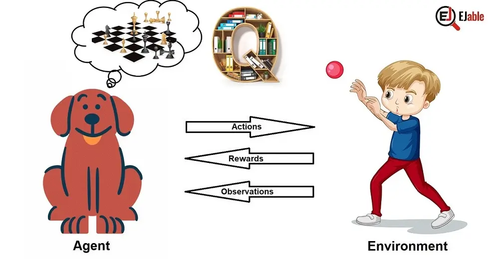
Imagine training a robot to navigate a maze. Now, think of teaching a computer to master chess. This is the realm where Q-learning becomes crucial.

Q-learning doesn’t give machines specific instructions on decision-making. Rather, it lets them learn from interactions and experiences. They navigate through choices using trial and error and continuously improve their strategies.

As we delve into Q-learning, we’ll explore how it enables machines to evaluate actions, comprehend reward-based learning, and, ultimately, choose paths that lead to success, one decision at a time.

As Q-learning is a type of reinforcement learning, it may be a good idea to read through the article about types of machine learning.

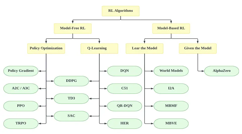
To recap, there are two types of Reinforcement Learning algorithms. These are as follows:

1. Model-free: This is a type of algorithm that estimates the optimal policy without using the dynamics of the environment. 
2. Model-based: This algorithm incorporates the dynamics of the environment (the transition and reward function) to estimate the optimal policy.

What is Q-Learning?

Q-learning is a model-free reinforcement learning algorithm randomly aiming to find the next best action to maximize the reward. It is a value-based learning algorithm that updates the value function based on an equation).

Given its current state, the Q-learning model aims to find the next best course of action. The Q-learning model operates on a somewhat liberating principle—it doesn’t strictly adhere to a pre-established set of rules or policies.

For the Q-model model to do this, it can generate its own rules or operate outside of its given policy. Therefore, this tells us there is no vital need for a policy. This is why it is known as an off-policy learner.

What is an Off-Policy Learner?

An off-policy learner means it learns the value of the optimal policy independent of the agent’s actions.

Delving into the term “off-policy learner,” it’s important to understand that this means Q-learning distinguishes itself by learning the value of the optimal policy, irrespective of the agent’s actual actions. At the same time, an on-policy learner learns the value of the policy carried out by the agent and finds an optimal policy. 

Q-learning continuously updates its value function based on a specific equation. It continuously adjusts and optimizes as it encounters new states and rewards. Each action taken and subsequent reward received enlightens the algorithm, enabling it to navigate through the complex web of decisions with an ever-increasing understanding of the outcomes.

This continuous, iterative process allows Q-learning to tread through the expansive universe of possible actions, incessantly seeking and ultimately homing in on the path that systematically maximizes its reward.

What does the ‘q’ in Q-Learning stand for? Well, the “Q” stands for “Quality.” It represents how effective a given action is in gaining rewards. 

An example of Q-learning is advertisements based on a recommendation system. Typically, advertisements pop up based on your search history or previous watches.

However, with Q-Learning, the model can optimize the ad recommendation system to recommend products frequently bought together. In this case, the reward signal will be generated if the user purchases or clicks on the suggested product.

Mathematics behind Q-Learning

Before we discuss further Q-learning, it’s essential to understand the mathematical backbone for the decision-making processes of our Q-learning model.

The mathematical equation behind q-learning is the Bellman Equation.

Q-learning, in its continuous efforts to find the optimal policy, leverages a systematic approach to quantify the quality, or ‘Q-value,’ of taking a specific action in a particular state.

The quest for precision and optimization of q-learning comes from the Bellman Equation. This equation is a mathematical expression that captures the relationship between the current value of a state and the potential future rewards that an action can yield.

Imagine a chess player thinking about his next move. Here, the value of his current position is intrinsically tied not only to the immediate consequence of his next move but also to its impact on future possibilities.

The Bellman Equation features this concept of a chess game. It establishes a looping or recursive relationship that ties the value of a current state and action to the anticipated rewards of subsequent states. This mathematical principle is a crucial feature of the Q-learning algorithm. This feature continuously propagates values backward from a rewarding future to earlier decisions.

The Q-learning algorithm applies the Bellman Equation iteratively, continuously refining the Q-values associated with state-action pairs.

As the agent explores its environment, it uses the Bellman Equation to update its estimates, calculating and recalculating Q-values to uncover new ways, experiences, and varied outcomes. Thereby, it learns more about the environment’s reward structure.

Thus, the Bellman Equation stands as a bridge, elegantly connecting immediate actions with future rewards and enabling Q-learning models to navigate complex decision-making processes with the foresight to find optimal policies.

Bellman Equation

Here’s a simplified expression of the Bellman equation for Q-learning:

Q(s,a)=r+γmax_a′​Q(s′,a′)

Where:

• “s” is the current state.
• “a” is the action taken in state “s”.
• “r” is the immediate reward received after taking action “a” in the state “s”.
• “γ” is the discount factor, which models the agent’s consideration for future rewards. It’s a value between 0 and 1, where a value close to 0 makes the agent short-sighted and primarily focused on immediate rewards, while a value close to 1 makes the agent prioritize long-term rewards.
• “s′” represents the subsequent state resulting from taking action “a” in the state “s.”
• “a′” represents a possible action taken in the state “s′”.
• “max_a′​Q(s′,a′)” represents the maximum Q-value achievable in the subsequent state “s′”, considering all possible actions “a”.

Further Explanation of the Calculation

Let’s say that we know all the expected rewards for every action. So, how do we determine which action to take? We can choose the sequence of actions that may generate the best rewards, referred to as the “Q” value. From this, we can then formulate it into this equation:

• Q(s, a) stands for the Q Value yielded at state ‘s’ and selecting action ‘a’. 

• This is calculated by r(s, a), which is the immediate reward received + the best Q Value from state ‘s.’ 
• γ is the discount factor that controls and determines the importance of the current state

The Bellman Equation was named after Richard E. Bellman, known as the father of Dynamic programming. Dynamic Programming is a class of algorithms that aims to simplify complex problems/tasks by breaking them down into sub-problems and recursively solving them. 

The Bellman Equation determines the value of a particular state and concludes how valuable it is in that state. The Q-function uses the Bellman equation and two inputs: the state (s) and the action (a).

This is the equation breakdown:

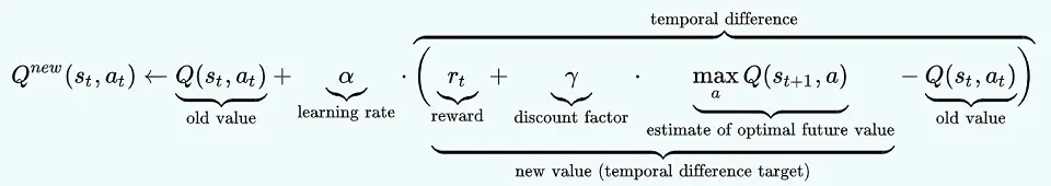
The equation uses the current state, the learning rate, the reward linked to that particular state, the discount factor, and the estimate of optimal future value (the maximum expected reward) to find the next state of the agent. The learning rate determines how fast or slow the model will be learning. 

What is a Q-table?

The point of Q-learning is that it will do what it wants, taking multiple paths and going through different solutions. But how do we determine which is the best? This is where the Q-table comes in. 

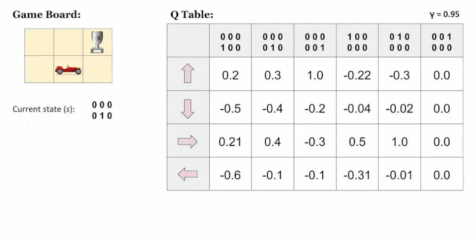
Q-table is really just a fancy name for a simple lookup table. It is created to calculate the maximum expected future rewards, finding the best action for each state in the environment. Using the Bellman Equation at each state, we get the expected future state and reward, then save it in a table to compare to other states. 

An example of a Q-table is as follows

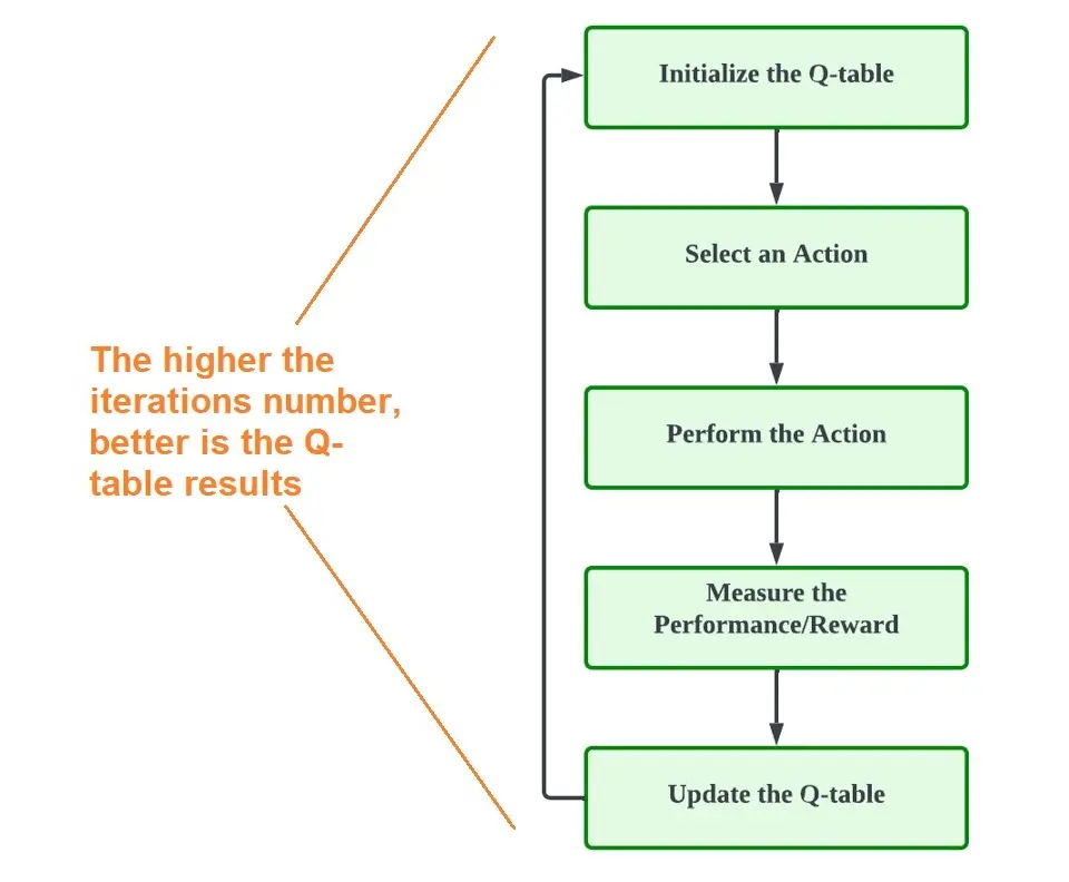
Q-Learning Process

So now that we know the elements of Q-learning, what is the process? Here is a breakdown.

1. Initialize the Q-Table

The first step is creating the Q-table, where:

• “n” represents the number of actions.
• “m” represents the number of states.

For example, “n” as an action may mean a move towards “left”, “right,” “up,” or “down,” while “m” may mean the status of the move, i.e., “start,” “idle,” “correct move,” “wrong move,” or “end.”

2. Choose, Perform and Action

In case no other action has been performed, our Q-table should have all 0’s. This is the start, so we choose an action, so let’s say we choose the action ‘up.’ 

We then update our Q-table in the start and up section, stating that the action has been performed. 

3. Calculate the Q-Value using the Bellman Equation

We now need to calculate the value of the actual reward and the Q-value for the action we just performed. We do this by using the Bellman Equation. 

4. Continue Steps 2 and 3

The agent will continue to take actions, and for each of these actions, calculation for reward and Q-values takes place to update the same in the Q-table. 

Steps 2 and 3 continue till an episode ends or the Q-table is filled. 

Q-Learning Applications

Here are some notable applications where Q-learning has been successfully employed:

1. Gaming and Game AI:
   • Board games like Chess and Go, where the algorithm can learn optimal strategies over numerous iterations.
   • Video games, such as those with complex environments and decision-making processes like StarCraft or Dota 2.
2. Robotics:
   • Navigation tasks, where a robot must learn to navigate through a space, avoiding obstacles.
   • Manipulation tasks, where a robot arm learns to pick up, move, and interact with objects.
3. Control Systems:
   • Autonomous vehicles, from simple simulated environments to real-world driving, where the algorithm learns to make complex sequences of decisions.
   • Industrial automation, where robots learn to perform tasks such as assembly line work more efficiently.
4. Resource Management:
   • Managing resources in computer systems, like allocating bandwidth or computational resources adaptively.
   • Smart grid energy management, where the algorithm can balance supply and demand optimally.
5. Finance:
   • Portfolio management, using Q-learning to balance risk and return when constructing investment portfolios.
   • Algorithmic trading, where the agent learns trading strategies to maximize profit based on historical data.
6. Traffic Light Control:
   • Adaptive traffic signal timing, where the system learns the best light change times to minimize waiting times and improve traffic flow.
7. Personalized Recommendations:
   • Adaptive websites and applications that learn from user interactions to personalize content and recommendations in real time.
8. Healthcare:
   • Personalized medicine, where treatment plans are adapted over time for better outcomes based on patient response.
   • Rehabilitation robots that adapt to the needs and responses of patients.
9. Telecommunications:
   • Network routing, where the algorithm finds the optimal path for data packet transmission to improve network performance.
10. Supply Chain and Inventory Management:
    • Dynamic inventory control, optimizing stock levels and ordering processes in response to demand predictions.

Conclusion

Q-learning is a model-free reinforcement learning algorithm that seeks to find the best action given the current state. Moreover, It has the capability to compare the expected utility of the available actions without requiring a model of the environment.

Q-learning has the advantage of not needing a model of the environment, which makes it applicable in a wide variety of settings, particularly those where the model dynamics are difficult to capture or the environment is subject to change.

However, it can be limited by the size of the state space. Therefore, it may become infeasible for very large state spaces, and in some cases, a variation or extension of Q-learning might be more appropriate.

If you want to learn more about Reinforcement Learning, I highly recommend this book: Reinforcement Learning: An Introduction (2nd Edition) by Richard S. Sutton and Andrew G. Barto.