Using Linear and Logistic Regression in Machine Learning

Logistic Regression and Linear Regression are two fundamental statistical methods used for predictive modeling within the supervised machine learning framework.

Before discussing these two concepts, let’s discuss what regression is and the use of regression analysis in machine learning.

What is Regression

Regression in statistics refers to a type of predictive modeling technique that analyzes the relationship between a dependent (target) and independent variable(s) (predictor). It estimates the output value based on one or more input values, identifying trends in data and predicting numerical values.

Logistic and linear regressions are fundamentally supervised learning algorithms because they rely on labeled training data to learn the relationship between input and output variables.

Statistics and Machine Learning

Statistics furnishes the foundational framework for machine learning (ML), providing tools and methods to extract insights and understand data. It assists in designing algorithms, validating models, and making informed decisions in ML by quantifying the reliability and accuracy of the models, thereby enabling the development of systems that can learn from data and make predictions or decisions.

Machine learning is an amazing approach to computing where we try to create predictions or output based on data passed into it (input). Usually, we have models that are trained to perform simple tasks or solve problems. Some of those machine learning models are linear regression models and logistic regression models.

Linear and logistic regression are very simple for building machine learning models and can be applied to find relationships in data.

What is Linear Regression

Linear regression is a problem-solving technique categorized under supervised learning, where the model looks for a relationship between independent and dependent variables passed into it.

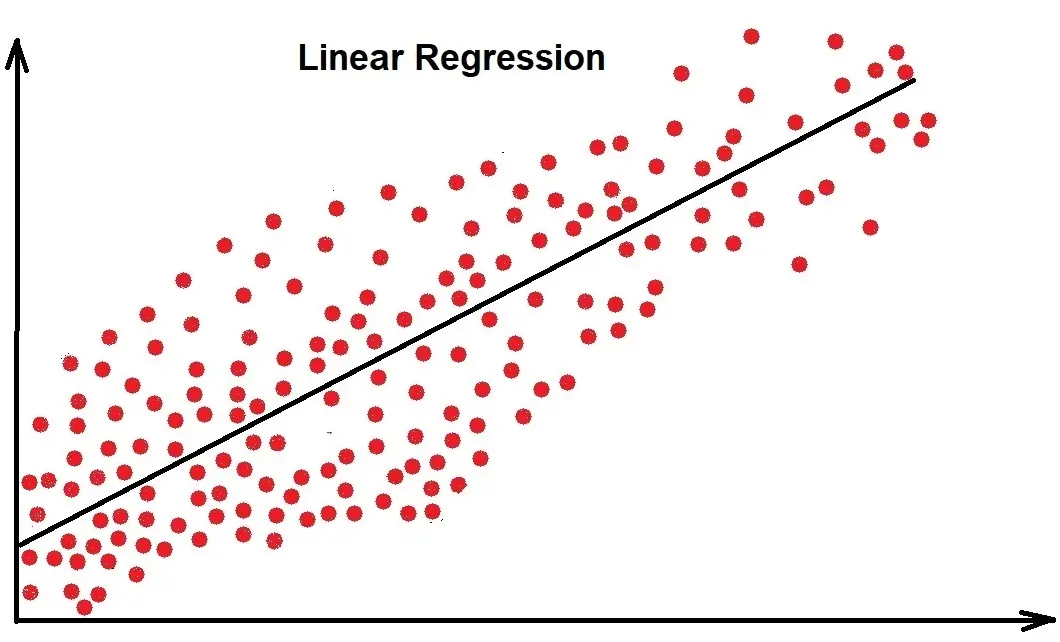
The concept of linear regression is to draw a single line of best fit. Here, best-fit means that the line is used to guess the value of the dependent value by passing in the independent values where we would have the smallest difference between the predicted value and actual value.

If we estimate the relationship between a single independent variable and one dependent variable using a straight line, we will class this as Simple Linear Regression. However, we call this Multiple Linear Regression if there are more than two independent variables. 

The Formula for Linear Regression:

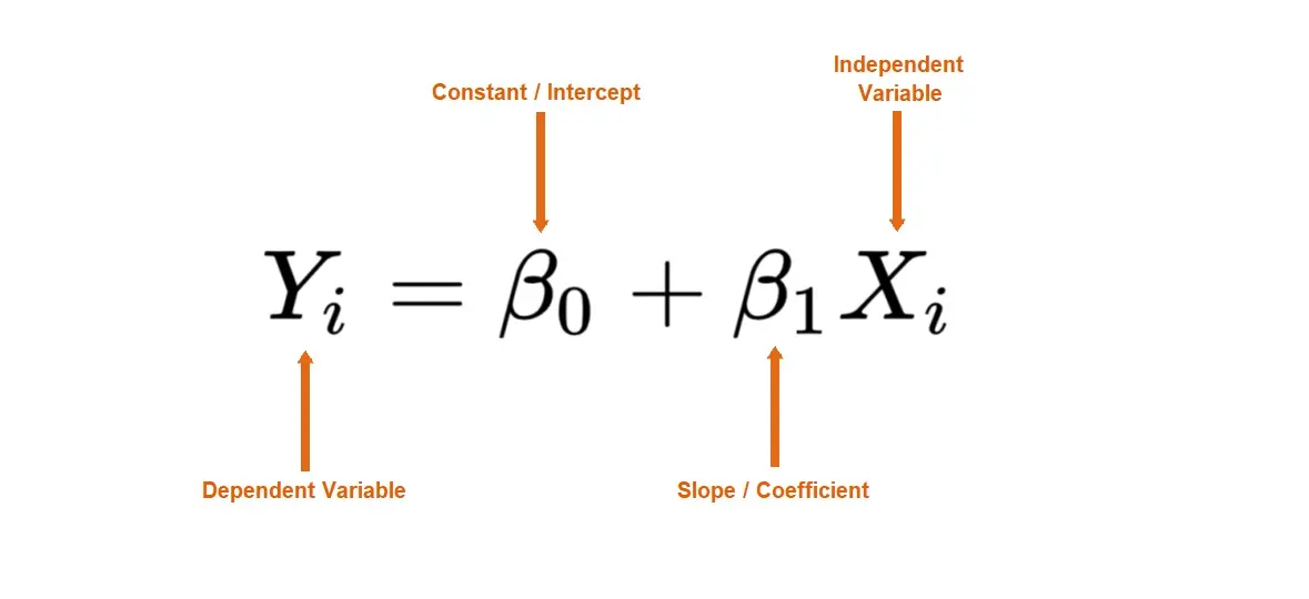
You may remember the formula: y = mx + b, which represents the slope-intercept of a straight line. ‘y’ and ‘x’ represent variables, ‘m’ describes the slope of the line, and ‘b’ describes the y-intercept, where the line crosses the y-axis. We can use this formula to interpret Linear Regression. 

The formula for Linear Regression is shown below.

The ‘y’ variable represents the dependent variable, the ‘x’ variable represents the independent variable, the “?0” variable represents the y-intercept, and the “?1” variable represents the slope, which describes the relationship between the independent variable and the dependent variable.

Example of Linear Regression Plot

The following plot shows the Best-fit straight line of a linear regression:

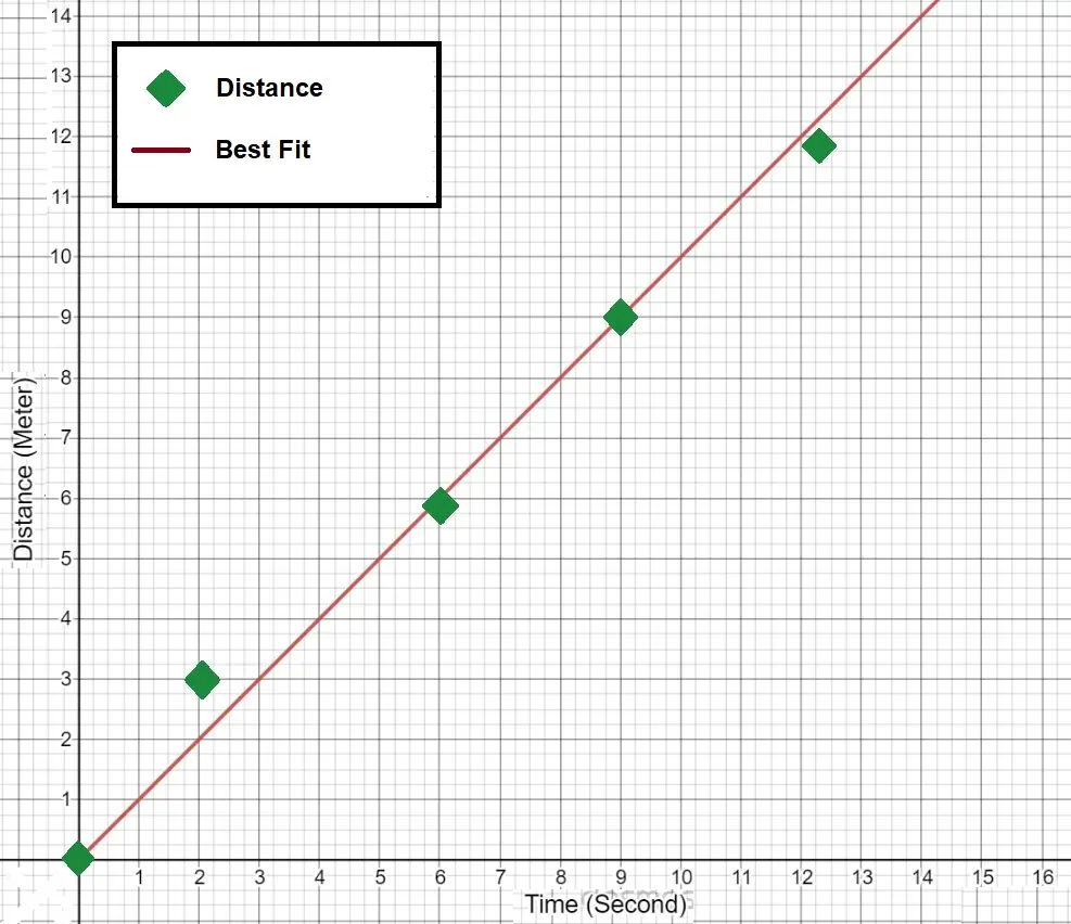
The equation of a straight line is Y = mX + b.

The equation of a straight line is given as the dependent variable y = (equals) to the product of the gradient and the independent value X +(plus) b, which is the starting point on the y-axis, the gradient being the slope or how bent our line is.

Two types of linear regression

• Simple linear regression: This involves when we have only one set of dependents in our equation

y = mx + b

• Multiple linear regression: This involves when we have multiple sets of dependent variables

y = m1x1 + m2x2 + m3x3 + m4x4 + m5x5 + m6x6 ………..+ b

b is the intercept on the y-axis and y being our dependent variable in both types of linear regression models.

Optimizing the values of our dependent variables

Our goal in optimizing the linear regression model is to find the best fit for the linear line that, when plotted on the graph, has the least total error by finding the best values of our independent values.

The distance between the data point and the point the regression line is on is known as error or residual.

Let’s look at the mathematics behind it, which is as follows;

• e = sum(y-y2)^2   
• y=actual_y – predicted_y   
• e = actual_value – predicted_value
• sum(e)
• square of sum = (sum(e))^2 

Assumptions Behind Linear Regression

The algorithm name also has ‘linear’ because it assumes a linear relationship exists between the input variables (features, x) and the output variable (target, y). Basically, it believes that y can be calculated from a linear combination of x. 

The above is one of the assumptions that the linear regression algorithm makes. 

All of the assumptions are:

1. Linearity – the relationship between a feature and the mean of the dependent variable is linear
2. Independence – each random sample (observation) is independent of one another 
3. Homoscedasticity – the variance of residuals (error = predicted – actual) is the same for any value of x (feature) 
4. Normality – for any fixed value of x (feature), y is normally distributed 

If any of the above assumptions are violated or not met, then the results from the model are redundant. This is also the main drawback of the linear regression algorithm since it is difficult for all these assumptions to hold “true” in the real world. 

Evaluating Accuracy of Model (Cost Function)

The point of every Supervised Learning algorithm is to learn from data and predict values or classes as correctly as possible so that the error/difference between the actual values and predicted values is the smallest it could be.

Linear Regression works the same way and uses this process of minimizing the error to find the best values for the coefficients.

We evaluate the accuracy of our model by calculating how far our predicted values are from our actual values. To perform this task, we have two options, which are the following:

MSE (Mean Squared Error)

Mean Square Error is the average value of the total error of all our data

MSE = |MSE| = (1/n)sum(y-y2)^2   

RMSE (Root Mean Squared Error)

Root Mean Square Error is defined as the root of the MSE value.

   |RMSE| = ((1/n)sum(y-y2)^2)^-2   

We need to know the errors. This enables us to be able to make changes to the values of our independent values.

The gradient descent algorithm finds coefficient values, which repeatedly updates the coefficient values by calculating the cost function, i.e., “Mean Squared Error (MSE)” or “Root Mean Square Error (RMSE).”

You may read more about MSE and RMSE in the article “Performance Metrics for Regression“.

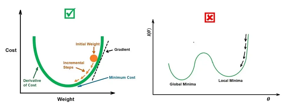
How does the gradient descent algorithm work?

Gradient Descent algorithm starts with some random values for a and b:

1. Calculates the cost function with those values — J(a, b)
2. Makes a small change in the values of a and b.
3. Calculates the gradient (change) in the cost function. If the gradient is smaller, repeat steps 2 and 3 until the gradient doesn’t change, meaning the graph has converged and the minimum has been reached.

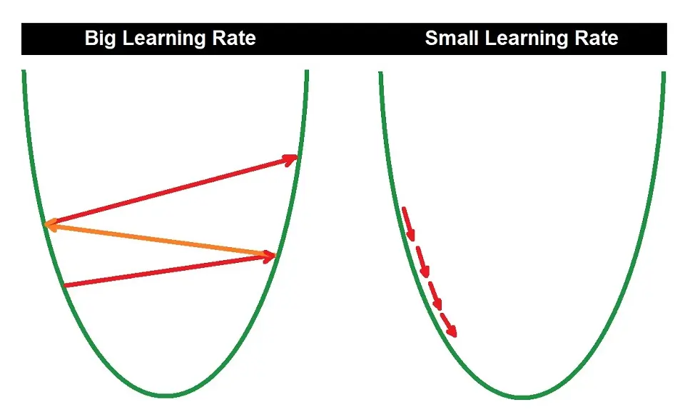
To understand this better, take a look at the U-shaped graph below. This represents the cost function. The gradient descent algorithm aims to reach the minimum point of this graph — it descends by taking steps.

The coefficient values to attain this minimum are the final values incorporated in the linear equation shown above and used to predict future values.

An important parameter that plays a role in the gradient descent algorithm is called the learning rate. The programmer specifies this and determines how many steps the algorithm takes to reach the minimum.

A small learning rate may take more time because it implies smaller steps, but a big learning rate might overshoot the minimum due to the large, few steps it implies. Hence, we need to find a good middle point.

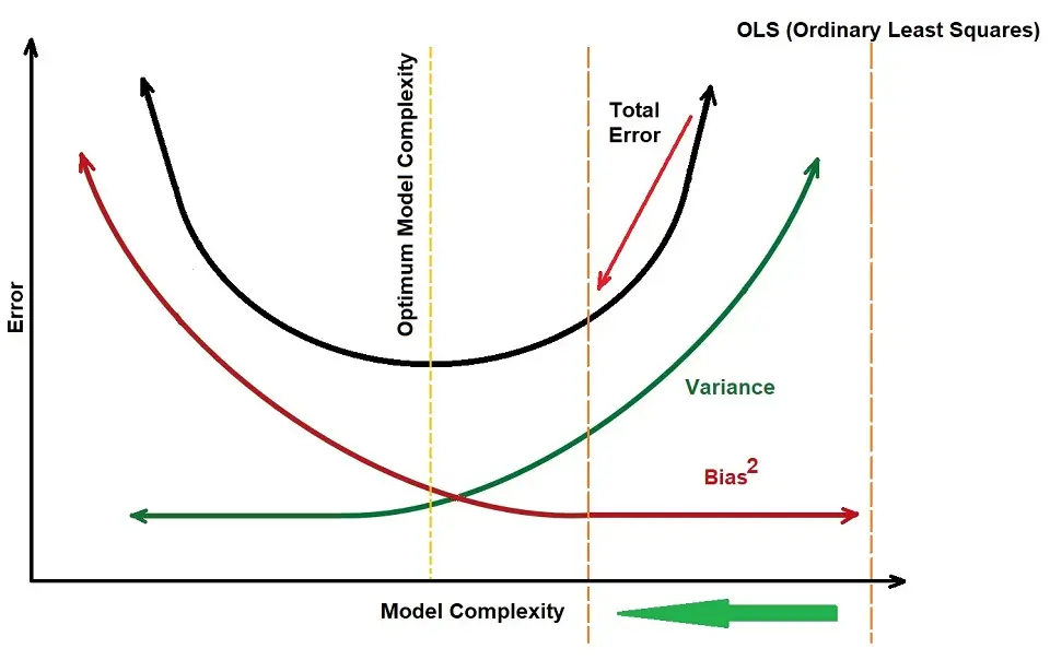
Linear regression models are pretty simple so they can lead to underfitting / a high bias. However, they can also overfit the data in some cases, so the concept of regularization is around to help us reduce the overfitting. 

There are three types of regularization with respect to linear regression:

1. L2 – Ridge Regression 

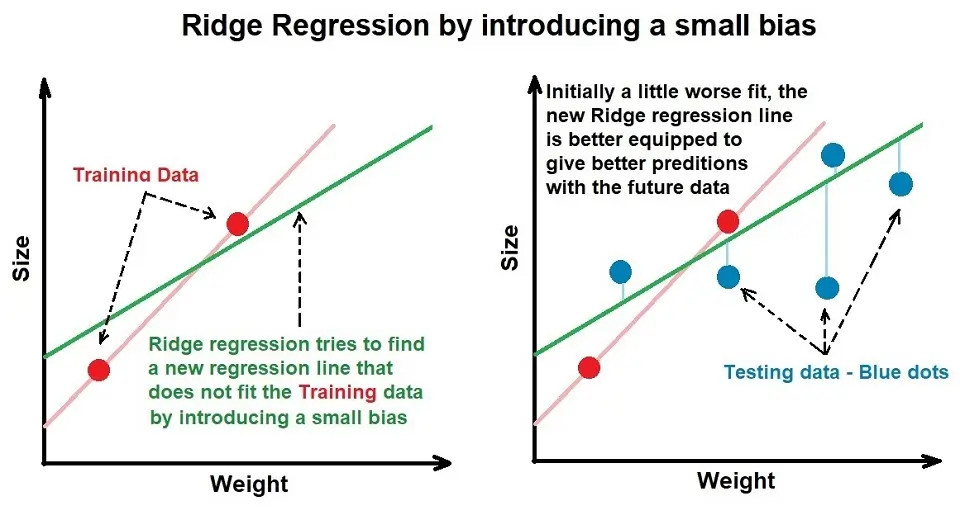
Ridge regression penalizes large model coefficients assigned to features. It involves a tuning parameter called lambda, which helps control the model’s flexibility.

Lambda multiplied by the value of the slope of the best-fit line squared is known as the ridge regression penalty. The higher the lambda, the more the model coefficients can approach 0, and the closer to 0 they are, the lesser importance that particular feature has on the output.

However, the model coefficients’ values can only approach 0 and never be 0. Hence, even if a feature isn’t impactful, it will still have a small model coefficient assigned to it and will be involved in the output prediction. 

2. L1 – Lasso Regression 

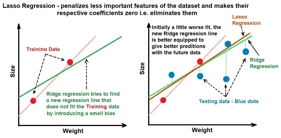
Lasso regression is like ridge regression, except instead of the ridge regression penalty, it uses the absolute value of the slope. The Penalty Function now is lambda*|slope|. It allows model coefficients of less important features to be 0 and performs feature selection on its own. 

3. Elastic net

The Elastic net is a combination of L1 and L2 regression. 

The elastic net method overcomes the limitations of the LASSO, including the LASSO and ridge regression, and falls between the latter two.

The main differences between these three regression methods are as follows:

• Lasso (L1): λ·|w|
• Ridge (L2): λ·w²
• Elastic Net (L1+L2): λ₁·|w| + λ₂·w²

Steps to Calculate Linear Regression

The name suggests the type of protocol we must follow to succeed in Linear Regression. It tells us that we must use a linear equation describing the relationship between dependent and independent variables.

Step 1:

Let’s assume we have a dataset where ‘x’ is the independent variable and Y is a function of ‘x’: represented as (Y=f(x)). We can then use the following equation: y = mx + b

Remember that ‘y’ and ‘x’ represent variables, ‘m’ describes the slope of the line, and ‘b’ describes the y-intercept.

Step 2:

To generate the line of best fit, we need to assign values to ‘m’, the slope, ‘b’, and the y-intercept. Thereafter, we calculate the corresponding values of ‘y’, the output, and ‘x’, the independent variable. 

As we use Linear Regression, we already know the actual value of ‘y’ because it is our dependent variable. 

Step 3:

Now, we have assigned a calculated output value to ‘y’. We can now verify if our prediction is correct or not. We can represent this output value as ‘ŷ’.

To calculate the accuracy of our prediction, we use the Cost/Loss Function. For Linear Regression, the Cost Function that we will use is Mean Squared Error (MSE) and is as follows: 

L = 1/n ∑((y – ŷ)2)

The value ‘n’ represents the number of observations. 

Step 4: 

To achieve the most accurate line of best fit, we have to minimize the value of our loss function. To do this, we use the Gradient Descent technique. 

We do this by taking the first-order derivative of the Cost Function for the weights denoted by ‘m’ and ‘b,’ our slope and y-intercept value, respectively. Thereafter, we subtract the result for that first-order derivative from the initial weight, which we multiply with a learning rate (α). We also use a small threshold value (for example, 0.001) to help us reach the exact zero value. 

We continue this process until we have reached the minimum value.

If you need a visual representation of the explanation of Gradient Descent, you can look at the image further in this article under the Cost Function and Gradient Descent section.

Step 5:

Once the Cost Function is the lowest, we can use this to get the final equation for the line of best fit, which will help us predict the value of ‘y’ for any given ‘x’.

Logistic regression

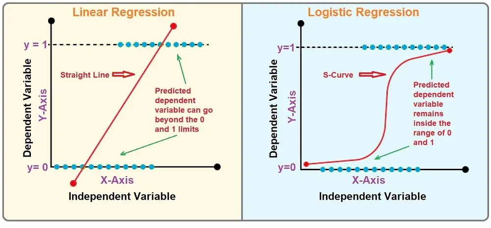
Logistic regression is a method of prediction to calculate the binary result of a set of inputs. By binary, we mean to say a situation where our answer is “yes” or “no.” We use It mainly in classification and outputs probability; its hypothesis or answers are always between 0 and 1.

Logistic Regression is based on probability and is used to predict the categorical dependent variable using independent variables. Logistic Regression aims to classify outputs, which can only be between 0 and 1. 

An example of Logistic Regression can be to predict whether it will snow today or not by using “0” or “1”, meaning a “yes” or “no,” or “true” or “false.” 

Logistics regression uses the sigmoid function to return the probability of a label. 

Type of Logistic Regression:

1. Binomial: There can be only two possible types of dependent variables, such as 0 or 1, Yes or No, etc.
2. Multinomial: There can be three or more possible unordered types of the dependent variable, such as “cat,” “dogs,” or “sheep.”
3. Ordinal: There can be three or more possible ordered types of dependent variables, such as “low,” “Medium,” or “High.”

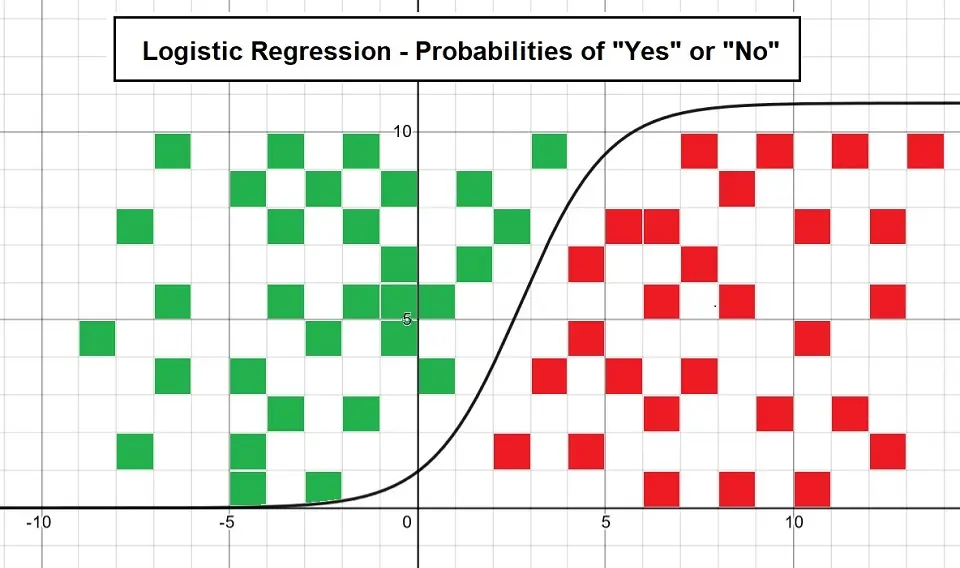
Example of Logistic Regression Plot

The following plot shows logistic regression by considering the probabilities of “Yes” and “No”:

Assumptions of logistic regression

• The output data is yes and no
• Linearity
• Little outliers
• Independence in value

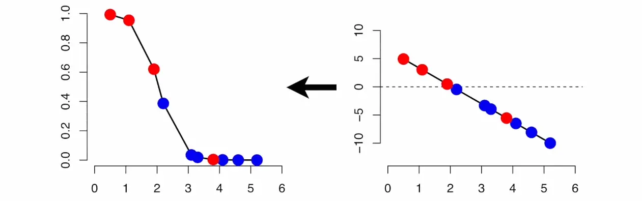
As we mentioned above, the answer to our logistic regression model is between 0 and 1. To ensure our output is at that value, we have to squash that data into that range. The best tool for doing this would be a sigmoid function.

Sigmoid Function

The sigmoid function is a mathematical function for mapping the predicted values to probabilities. The function can map any real value into another value within 0 and 1. 

Code of Sigmoid Function:

def sigmoid(z):
  return 1.0 / (1 + np.exp(-z))

A visualization of the Sigmoid Function is as below. Due to the limitations of being unable to go beyond the value “1” on a graph, it forms a curve in the form of an “S.” This is an easy way to identify the Sigmoid function or the logistic function.

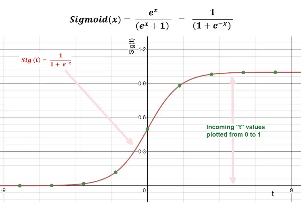
This works because we have an upper and lower limit of 1 and 0.

sigmoid = 1 / (1+e^-x)

our x value would equal our equation of a straight line

 X = b1 + b2x 

The “Loss Function” for Logistic Regression

From our experience with linear regression, our loss function represents how wrong our current model is. Moreover, it shows us what we must correct in what direction or how far.

Sadly, the cost function we discussed in linear regression cannot work for logistic regression because we would settle at the local maxima of our problem space.

We don’t want this to be our case.

A notable way of solving this is using Cross entropy (Log loss), which calculates the difference between two probability distributions. However, it is a fancy way of saying it calculates how wrong the probability guessed is Vs. the actual value and penalizes the model based on how wrong we are.

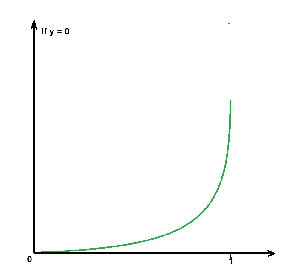
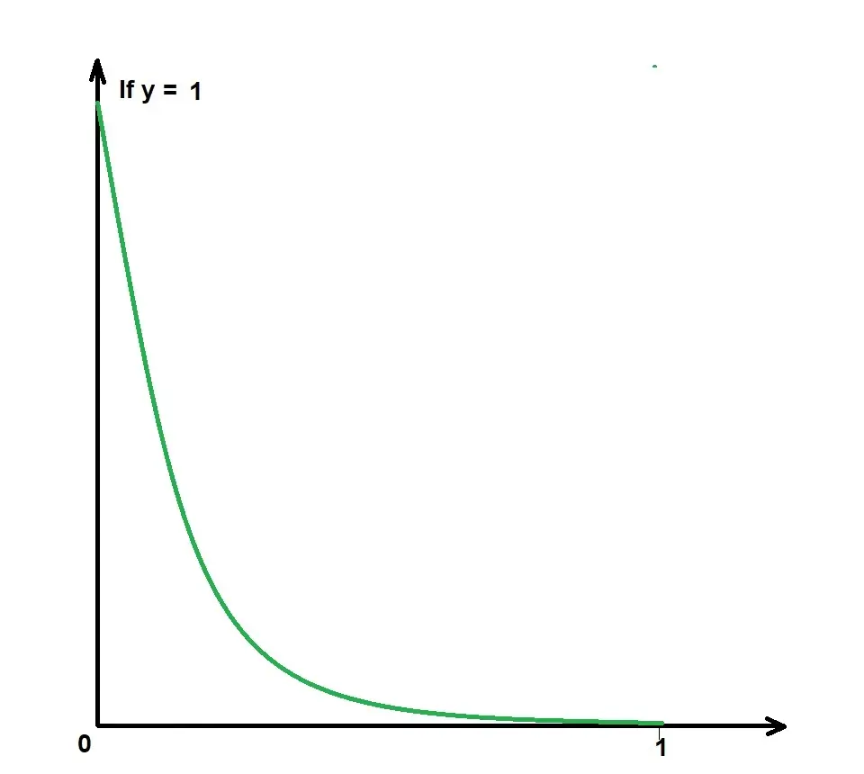
From the image, we handle data differently for values of y.

Y can only be 0 or 1, (not predicted y!!!).

 -log(p(x)) when (y =1) 

 -log(1-p(x)) when (y =0) 

We can simplify these two equations into one equation:

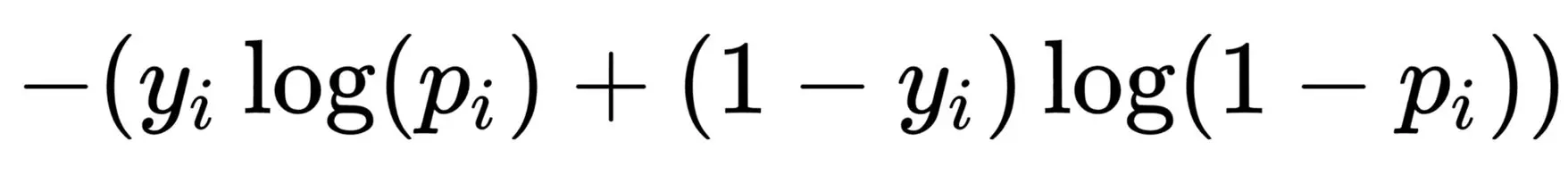
When we substitute y with 1 in the following equation:

-log(p(x)) 

Then, when we substitute y with 0 in the equation, we have the following:

-log(1-p(x)) 

Now, we can substitute the value into our RMSE (Root Mean Square Error) value that we previously declared.

Root Meen Square Foot (RMSE) Formula

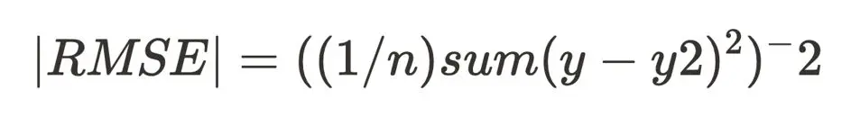
but substitute the y^2 value for our defined equation

we would end up with the equation below

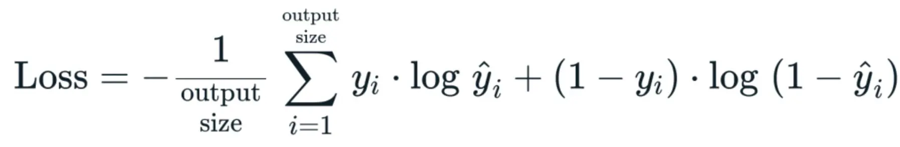
Simple right?

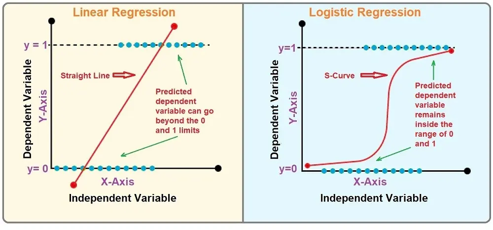
Linear Regression Vs. Logistic Regression

Logistic regression and linear regression are both very different solutions for different problems. With logistic regression, we can solve very basic “yes” and “no” questions, e.g., is someone “happy” or “sad,” “sick” or “healthy.”

On the other hand, linear regression is good for solving problems where the values have continuous values, which means no upper and lower limits (cap if you will have to throw this in here).

These are two types of problems and different ways to solve them, but we can optimize both with similar algorithms like gradient descent.

The following table summarizes the comparison of linear and logistic regression:

Linear Regression	Logistic Regression
Linear regression predicts the categorical dependent variable using a given set of independent variables.	Logistic regression predicts the categorical dependent variable using a given set of independent variables.
The outputs produced must be of a continuous value, such as price and age.	The outputs must be categorical values such as 0 or 1, True or False.
Linear regression is primarily used for solving Regression tasks.	Logistic regression is primarily used for solving Classification tasks.
We use the best-fit line to help us easily predict outputs.	The relationship between the dependent and independent variables DOES NOT need to be linear.
In Linear regression, the relationship between the dependent and independent variables must be linear.	The relationship between the dependent and independent variables DOES NOT need to be linear.
We use the best-fit line to help us easily predict outputs.	We use the S-curve (Sigmoid) to help us classify predicted outputs.
The mean squared error method is used for the estimation of accuracy.	The cross-entropy method is used for the estimation of accuracy.
There is a possibility of collinearity between the independent variables.	There should not be any collinearity between the independent variables.

Visual representation of the difference:

Visual representation of Linear Regression being transformed into Logistic Regression:

When to Use Linear or Logistic Regression?

When to use linear regression and when to use logistic regression based on the type of problem you are trying to solve and the nature of the data you are working with. A deep dive on their use is as follows:

When to Use Linear Regression:

Use linear regression when dealing with a continuous outcome variable, and you want to predict where it falls on a continuum. It is most appropriate in the following situations:

• Predicting Quantity: Linear regression is ideal for predicting quantities, such as forecasting sales, assessing the number of calls to a call center, or estimating electricity consumption.
• Relationship Analysis: When you want to understand the strength and direction of the relationship between independent (predictor) variables and a dependent (outcome) variable.
• Homoscedasticity: The residuals (i.e., prediction errors) should be the same across all levels of the independent variables.
• Parametric Assumptions: Your data should be linearly related, and you should confirm that it meets the assumptions required for linear regression, such as linearity, independence, and normality.

When to Use Logistic Regression:

Use logistic regression when your outcome variable is binary or categorical and you want to estimate the probability that a given input point belongs to a certain class. Consider logistic regression in these scenarios:

• Binary Outcomes: Logistic regression is the go-to method for binary classification problems, such as spam detection, churn prediction, and diagnosing diseases.
• Probability Estimates: If you need to measure the probability or risk of a particular event happening based on the log odds.
• Non-Linear Boundaries: Logistic regression can handle non-linear effects more naturally because it doesn’t assume a linear relationship between the independent and dependent variables.
• Understanding Impact: When you want to understand the impact of several independent variables on a single outcome variable.

Concluding Note about Linear and Logistic Regression

In essence, the decision to use linear or logistic regression comes down to the type of question you’re trying to answer.

Opt for linear regression when you aim to predict a continuous variable—such as temperature, prices, or scores—and your main objective is to determine the effect size of the predictors.

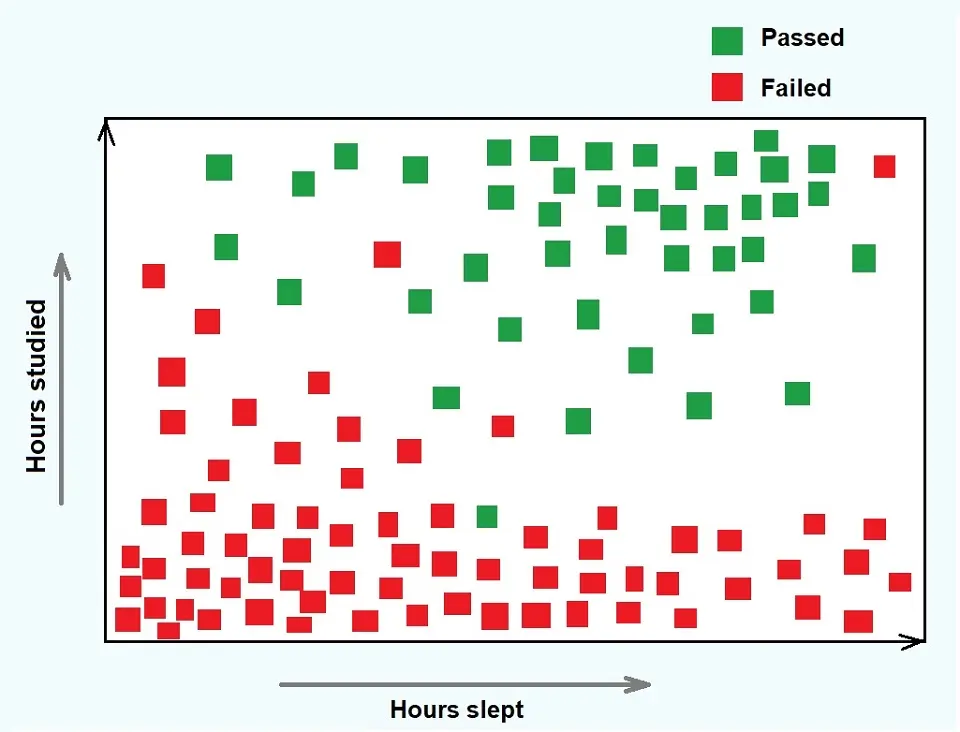
Turn to logistic regression when you aim to predict categorical outcomes, like pass/fail, win/lose, or healthy/sick, particularly when you’re interested in the odds or probabilities of occurrence.

The key is to match the regression technique to your data’s structure and the nature of the outcome variable. By carefully considering these aspects, you ensure that the insights and predictions you glean from your analysis are robust and meaningful.

You may also like to check the Performance Metrics for Regression in Machine Learning article.