Performance Metrics for Regression Problems in Machine Learning

Performance metrics are numbers that help measure the efficiency of your machine-learning algorithm and determine whether it’s solving the problem correctly. They also help compare and evaluate different algorithms for the same use case and determine which one you should go ahead with.

The decision of which performance metric to use for your machine learning problem first depends on the type of problem itself, as there are different sets of metrics for classification and regression problems (due to the difference in outputs). 

This article will discuss the various performance metrics available for regression problems and their strengths and drawbacks. 

1. Mean Squared Error (MSE)

Mean Squared Error (MSE) or Mean Squared Deviation (MSD) is a performance metric widely used for regression problems in machine learning. It measures the average of the squares of the errors—that is, the average squared difference between the actual value of an observation and the value your model predicted.

As the name states, this metric is the square of the average of the errors of your model. Error is the difference between the actual value of an observation and the value your model predicted.

For example, if your model predicts age and the actual age of point X is 23, but your model predicted 21, then the error = 23 – 21 = 2. Therefore, the squared error is 2² = 4. 

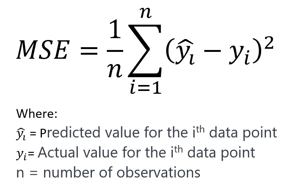
The Formula for MSE:

The MSE is calculated as the mean value of the squared differences between the model’s predicted values and the dataset’s actual values. 

The following picture shows the formula of the Mean Squared Error (MSE) or Mean Squared Deviation (MSD):

Properties of MSE:

• Since this metric involves squaring errors, it can never be negative.
• MSE is rarely “0” since there is always some noise in real-world data.
• Mean is a measure of central tendency that is not robust to outliers (because one arbitrary value can significantly impact the mean); hence, this performance metric is also not robust to outliers.
• The metric is in the square unit of the dependent variable. For example, in the above age example, the error measure is in years squared, whereas the model output is in years.
• Big errors are penalized, but smaller ones are also. Therefore, it leads to overestimating the model’s performance.

Interpretation of MSE:

• MSE is always non-negative, and values closer to zero are better. A zero value indicates perfect predictions without any error, which is an ideal but often unattainable situation in practice.
• MSE penalizes larger errors more than smaller ones due to the squaring of each term. This means that larger mistakes result in more significant increases in MSE, highlighting the presence of outliers or large deviations in predictions.
• The square root of MSE yields the Root Mean Squared Error (RMSE), which is on the same scale as the target variable and can sometimes be more interpretable.

Pros of MSE:

• MSE is very popular and easy to understand and implement.
• It provides a smooth and differentiable function, which is convenient for optimization using gradient descent and other techniques.
• It heavily penalizes significant errors, which can be desirable when they are undesirable in the application domain.

Cons of MSE:

• The heavy penalization of large errors means that MSE is not robust to outliers. MSE can give a skewed picture of model performance in datasets with significant outliers.
• Because the errors are squared before they are averaged, the MSE does not indicate the direction of errors (i.e., overestimation vs. underestimation).
• It assumes that the errors are homoscedastic, meaning they are evenly distributed across the regression line. When this assumption does not hold, MSE can be misleading.

Applications of MSE as Performance Metrics:

MSE is appropriate in contexts where large errors are undesirable and should be penalized more severely. Therefore, it finds wide use in many fields, from financial forecasting to environmental modeling, wherever regression analysis is performed.

In summary, while MSE is a fundamental performance metric for regression problems, its appropriateness depends on the specific context and characteristics of the data being modeled. Understanding the implications of the metric and considering complementary metrics can provide a more holistic evaluation of a regression model’s performance.

2. Root Mean Squared Error (RMSE)

Root Mean Squared Error (MSE) is also called Root Mean Squared Deviation (RMSD). RMSE is built on top of MSE,

The Root Mean Squared Error (RMSE) is a standard way to measure the error of a model in predicting quantitative data. It is the square root of the Mean Squared Error (MSE) and measures the magnitude of the error in the same unit as the output variable.

Taking the square root helps solve a lot of the drawbacks faced with MSE: 

• The metric is in the same unit as the dependent variable.
• Large errors are highly penalized.
• The penalization of minor errors is to a lesser degree.
• Less prone to outliers.

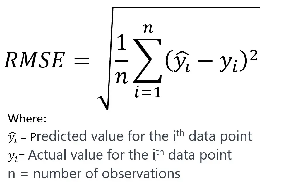
The Formula of RMSE:

RMSE is calculated as the square root of the mean of the squared differences between the predicted values and the actual values using the following formula:

Interpretation or RMSE:

• Like MSE, RMSE is always non-negative, and a lower RMSE is better.
• RMSE is expressed in the same units as the target variable, making it more interpretable than MSE.
• It penalizes larger errors, which can be useful when significant errors are undesirable.

Pros or RMSE or RMSD:

• The scale of RMSE is the same as the data, making it easier to understand the magnitude of the errors.
• It maintains the desirable properties of MSE, being differentiable and thus suitable for optimization.
• Large errors disproportionately impact RMSE, so it’s useful when you want to penalize larger discrepancies more.

Cons of RMSE:

• RMSE also is not robust to outliers; a few large errors can dominate the error metric.
• Like MSE, RMSE does not indicate whether the model underestimates or overestimates the target variable.
• RMSE assumes that the distribution of the residuals is normal, which might not always be true.

Applications of RMSE as Performance Metrics:

RMSE finds wide use in many predictive modeling contexts, such as weather forecasting, stock market prediction, and energy demand modeling. It is particularly useful in contexts where you want to know the error magnitude on the same scale as the data you’re modeling.

The use of RMSE in reporting model performance is often with other metrics, such as Mean Absolute Error (MAE) or Mean Absolute Percentage Error (MAPE), to provide a more complete picture of model accuracy.

3. Mean Absolute Error (MAE)

Mean Absolute Error (MAE) is another common metric to evaluate the performance of regression models in machine learning. It quantifies the average magnitude of the errors in a set of predictions without considering their direction.

MAE is the mean value of absolute errors (the definition of error is the same as that in MSE, i.e., error = actual – predicted). The absolute value is taken for each error, and all the absolute values are added together. This total is divided by the total number of observations. 

For example, if you have three observations as follows, then their absolute values will be |actual – predicted|:

Observation	Actual Age	Predicted Age	Absolute Value
A	23	21	|23 – 21| = 2
B	24	22	|24 – 22| =2
C	21	22	|21 – 22| = 1

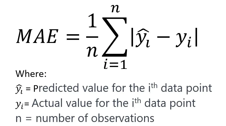
Formula to Calculate MAE:

MAE is calculated as the average of the absolute differences between predicted and actual values. Following is the formula to calculate Mean Absolute Error (MAE):

Properties of MAE:

• Absolute values are always positive since they disregard the sign of a number (+ or -).
• Due to the above property, MAE does not consider the direction of the error. Instead, it only calculates the distance between the actual and predicted values.
• Since the errors are not squared, large errors are penalized linearly, not exponentially, as each error contributes to the total error in proportion to its absolute magnitude.
• Like RMSE, the metric is in the same unit as the dependent variable.
• It is more robust to outliers.

Interpretation of MAE:

• MAE takes the absolute value of each error before averaging. Thus, it measures the average magnitude of the errors in a prediction set.
• It’s a linear score, which means all the individual differences are weighted equally in the average.
• A lower MAE is better, with 0 indicating no error (perfect predictions).

Pros of MAE:

• MAE is easy to understand and interpret since it’s in the same units as the output variable.
• It is less sensitive to outliers than MSE or RMSE because it doesn’t square the errors.
• As a result, it gives a more robust indication of the average error over a set of predictions.

Cons of MAE:

• Since MAE does not square the errors, it may not sufficiently penalize large errors, which could be particularly problematic in some contexts where large errors are very undesirable.
• It does not give any insight into the direction of the errors (whether the predictions are under or over-estimates).
• It may not be as useful for gradient-based optimization methods because the gradient of MAE can be the same throughout (since it does not depend on the magnitude of the error), which may result in convergence issues.

Applications of MAE as Performance Matrics:

MAE is commonly used in finance, weather forecasting, sales forecasting, and any domain where the magnitude of the prediction errors should be directly comparable. It is particularly useful we expect the distribution of error magnitudes to be uniform rather than focusing on penalizing larger errors. It’s also a useful metric when outliers are expected but are not the primary concern.

4. Mean Absolute Percentage Error 

Mean Absolute Percentage Error (MAPE) is a metric to measure the accuracy of a forecasting model as a percentage. It represents the average absolute percent difference between predicted and actual values for all observations.

MAPE metric is similar to MAE, except each absolute value of an error is divided by the actual value so that it is converted into a percentage. 

Using the same example as in MAE, the absolute percentage error would be | (actual – predicted) / actual|: 

Observation	Actual Age	Predicted Age	Absolute Value	Absolute Percentage Error
A	23	21	|23 – 21| = 2	2 / 23 = 0.087
B	24	22	|24 – 22| = 2	2 / 24 = 0.083
C	21	22	|21 – 22| = 1	1 / 21 = 0.048

All the absolute percentage errors are added together, and then the total is divided by the number of observations to get the MAPE (Mean Absolute Percentage Error. 

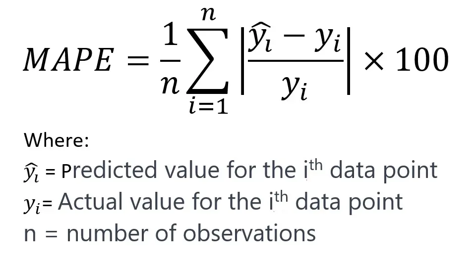
Formula for MAPE

MAPE is calculated as the average of the absolute percentage errors between predicted and actual values. The formula for MAPE is as follows:

Interpretation of MAPE:

• The MAPE expresses error as a percentage, making it easy to interpret and understand.
• It is scale-independent, allowing for comparing datasets with different scales.
• A lower MAPE value indicates better predictive accuracy, with 0% being the ideal.

Pros of MAPE:

• Provides an intuitive percentage-based measure that is easy for non-technical stakeholders to understand.
• MAPE is good for comparing the forecasting accuracy of different models or datasets that are on different scales.

Cons of MAPE:

• MAPE can be significantly skewed by zeros or very small denominators in the actual values (��yi​).
• MAPE can be undefined if actual values are equal to zero, a limitation for datasets where zero is a valid or common value.
• The measure can also be infinite or highly sensitive to small changes near zero, which is not ideal for practical applications.

Applications of MAPE as Performance Metrics:

MAPE finds wide use in various domains, such as finance for forecasting stock prices, sales forecasting, demand forecasting, and any predictive modeling task where percentage errors are a meaningful metric.

MAPE is particularly useful in business contexts for planning and monitoring where forecasts are communicated regarding percentage errors. However, due to its limitations, especially in dealing with zero or near-zero actual values, it may not always be the best choice. Therefore, you may prefer alternative metrics like MAE or RMSE.

5. R-Squared / Coefficient of Determination (r²)

The R-squared value is also known as the coefficient of determination. It is a statistical measure representing the proportion of the variance for the dependent variable explained by the independent variables in a regression model.

The R-squared metric differs from those previously discussed because it does not concern itself directly with the average values. Instead, R-squared quantifies the proportion of the variance in the dependent variable that is predictable from the independent variables in the regression model. So, in terms of the features and output – we need to check the following:

• Variance in the dependent variables
• Variance in the feature variables

And then check how much of the variance in the dependent variables can be explained by that of the feature variables.

For example, if the value of r² is 63% (or 0.63), we can say that the variance of the model’s feature is 63%. 

R² is between 0 and 1 (or 0 and 100%). The higher the value of r², the better it is (closer to 1). A higher value means that more of the variance of the dependent variable is explained by the features used to create the model, which is what you want.  

Formula for r² (R-Squared)

R-squared is the ratio of the variance explained by the model to the total variance in the data. The formula to calculate Squared-R Performance metrics is as follows:

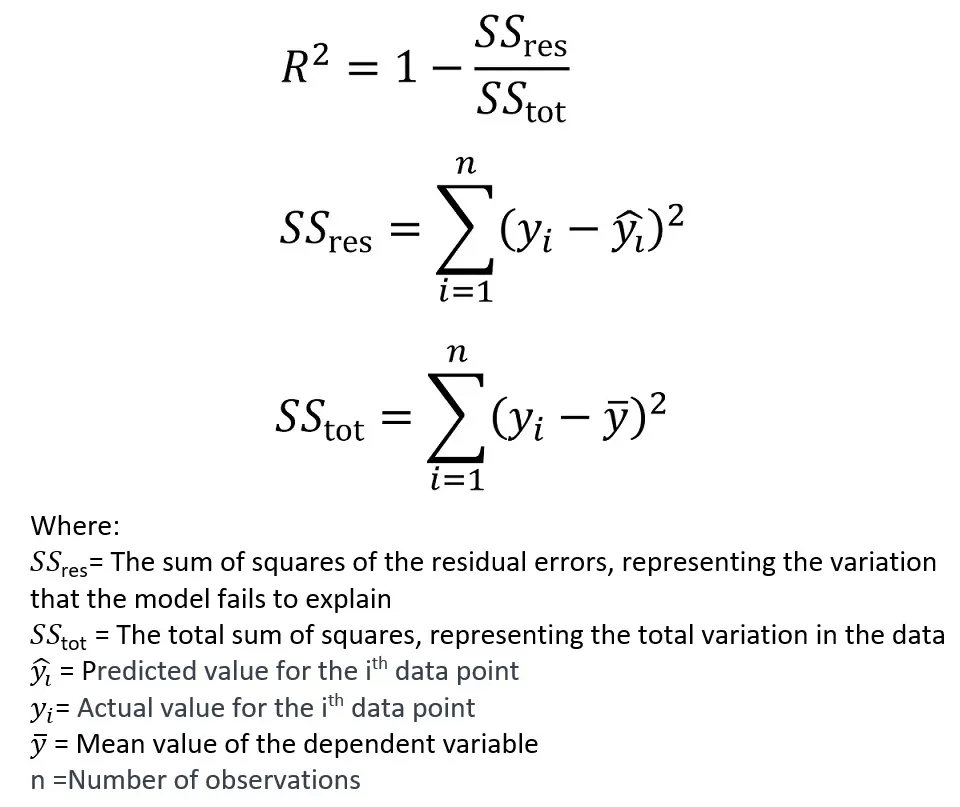
Interpretation of R-Squared:

• R-squared values range from 0 to 1.
• An R-squared of 1 indicates that the regression predictions perfectly fit the data.
• An R-squared of 0 means that the model does not explain any of the variability of the response data around its mean.
• While a higher R-squared is generally better, it is not a definitive measure of model quality because a model with more predictors can have a higher R-squared simply because it’s more complex, not necessarily because it has better predictive power.

Pros of Squared-R:

• R-squared is easy to interpret and explain to non-technical audiences.

Cons of Squared-R:

• R-squared can give a falsely high value if the model is overfitted. In such a case, it looks good on the training data but doesn’t generalize well.
• It does not consider the number of predictors in the model compared to the number of observations, which can be addressed by the adjusted R-squared.

Applications of R-Squared as Performance Metric:

R-squared is a common measure for the goodness of fit in linear regression, logistic regression, and various other modeling approaches where you want to quantify how well your model explains the variance in your dependent variable. It’s frequently used in fields like economics, psychology, environmental science, and any domain where regression models are common.

6. Adjusted R-Squared

The Adjusted R-squared is a modified version of R-squared to overcome the drawback of R-squared. This metric is adjusted for the number of predictors in the model. It is particularly useful when comparing models with a different number of independent variables.

The Adjusted R-squared considers the actual features rather than just the number of features. So, if redundant or unimportant features are added to the model, adjusted r² decreases. But if essential and relevant features are added to the model, then adjusted r² increases. 

The Formula for Adjusted R-Squared:

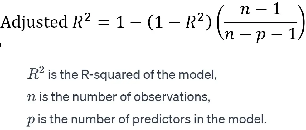
Interpretation of Adjusted R-squared:

• Adjusted R-squared penalizes for adding predictors that do not improve the model.
• A higher Adjusted R-squared indicates a better model that explains more variability of the response data with fewer predictors.
• Unlike R-squared, the Adjusted R-squared can decrease if useless predictors are added to the model.

Pros of Adjusted R-squared:

• Adjusted R-squared provides a more accurate measure of the goodness of fit, especially when comparing models with a different number of predictors.
• It helps to prevent overfitting by penalizing the addition of non-significant variables.

Cons of Adjusted R-squared:

• Adjusted R-squared can still lead to overfitting if too many predictors are included, and it’s not a substitute for proper cross-validation or other model validation techniques.

Applications of Adjusted R-squared as Performance Metrics:

Adjusted R-squared finds wide use in the same areas as R-squared as performance metrics for regression in machine learning. However, it is particularly favored when models are being compared with a different number of independent variables, such as in stepwise regression.