Introduction to Decision Trees in Supervised Learning

The Decision Tree algorithm is a type of tree-based modeling under Supervised Machine Learning. Decision Trees are primarily used to solve classification problems (the algorithm, in this case, is called the Classification Tree), but they can also be used to solve regression problems (the algorithm, in this case, is called the Regression Tree).

The concept of trees is found in graph theory and is used in computer science.

Decision Trees are Acyclic-Connected Graphs

Let’s break that definition down.

• Graph: A visual representation consisting of a finite set of nodes/vertices and two-element subsets called edges that form connections between the vertices.

• Connected graph: A graph in which every node has at least one connection to another node in the graph

• Acyclic graph: An Acyclic graph is a graph that does not contain a cycle.

Types of Nodes in Decision Trees

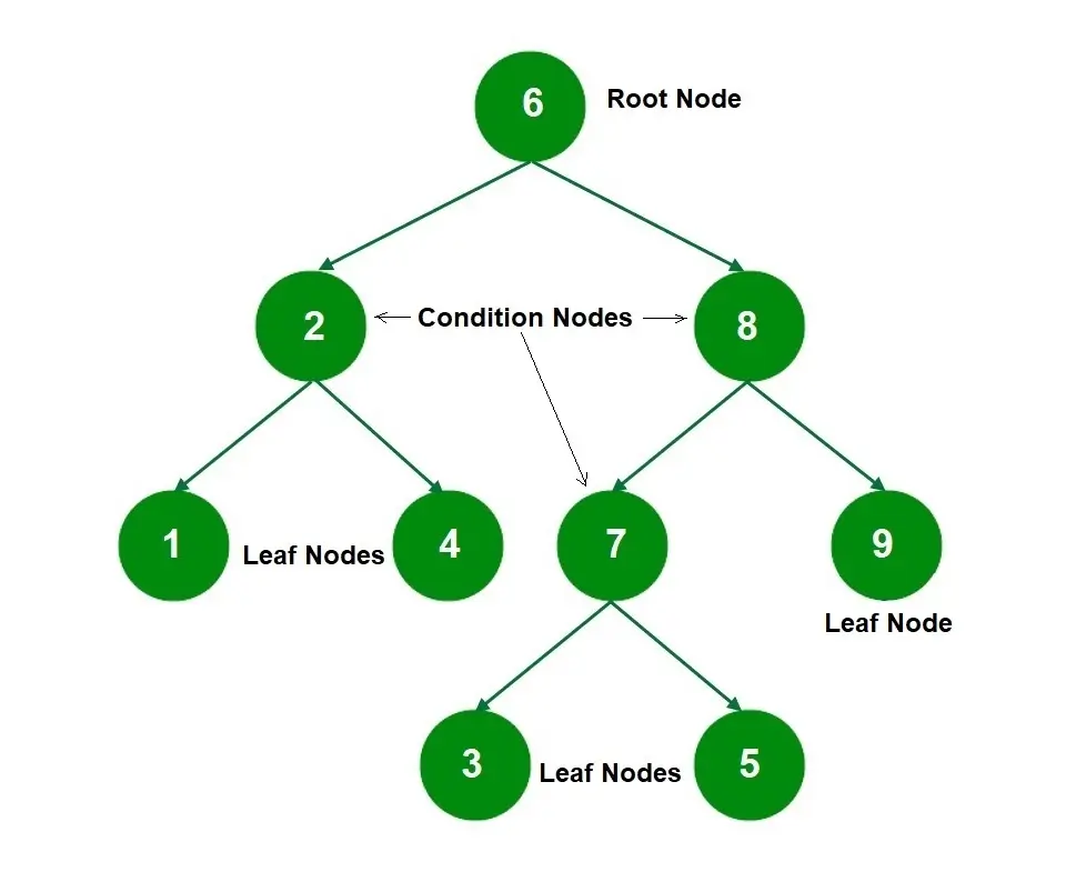
A decision tree has three types of nodes:

1. Root Node
   • This is the top node of the decision tree, also known as the Root.
   • The Root node represents the ultimate objective or decision you’re trying to make.
2. Internal Nodes or Condition Nodes
   • These branch off starting from the Root Node and represent different options.
   • They have arrows pointing to and away from them.
3. Leaf Nodes
   • These are attached at the end of the branches and represent possible outcomes for each action.
   • These have arrows pointing to them but not any arrows pointing away from them.

Explanation

So, in the case of the tree above, node 6 is the root node, nodes 2, 8, and 7 are condition nodes, and nodes 1, 4, 9, 3, and 5 are leaf nodes.

The features from the data set get translated into condition nodes in the decision tree. The process of determining which feature will be the first condition node and then breaking the tree further into more sub-branches is known as splitting. The aim of splitting is for the proceeding node to have a set of homogeneous data points — that is, similar data points.

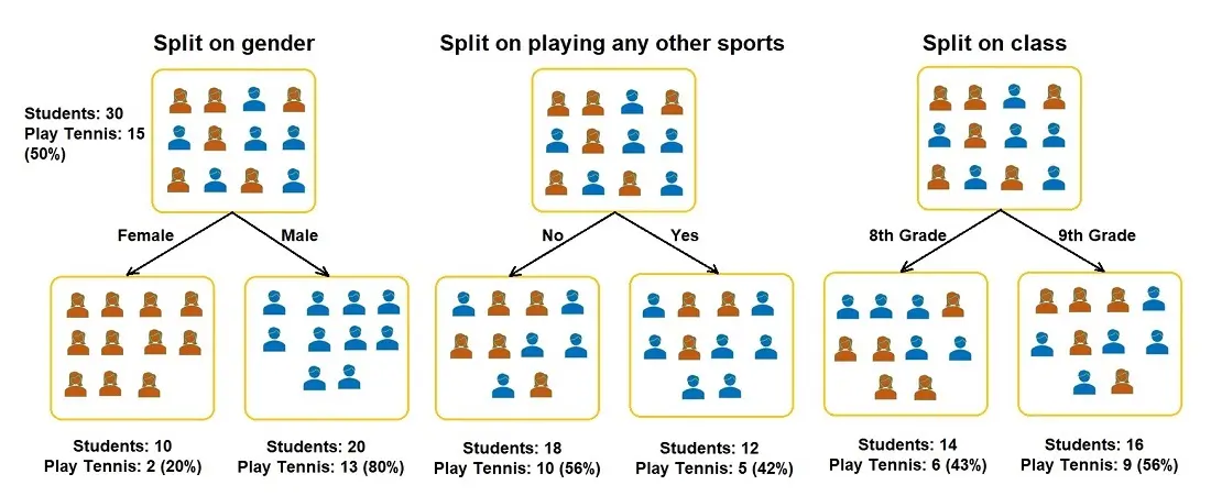
For example, you have a group of 30 students, with 10 girls and 20 boys, and you want to segregate the students based on whether they play tennis (there are 15 total). Other features included are the students’ class (8^th or 9th grade) and if they play another sport (yes or no). The splitting process now has to determine which feature should be the first condition node so that two homogeneous sets are produced. Let’s see how the groups look when the students are split on the three features.

Decision Tree Algorithm

But how does the algorithm decide which features to use, which order to use, and when to stop?

It uses the concept of Recursive Binary Splitting.

The algorithm tries each split on each feature and calculates the cost of each split using a cost function. Finally, the split that produces the least cost is chosen.

It does this repeatedly, hence ‘recursive,’ and this is also why this is a greedy algorithm (an algorithm that chooses the option that seems best at that moment, kind of like making a decision based on short-term benefits rather than long-term benefits).

The cost function aims to arrive at homogeneous groups — groups that have the most similar responses. We saw this in the above example of segregating students who play the piano. So, the decision tree splits the data on all the available features and then decides which one is the best choice based on the homogeneity of the sub-nodes that are produced.

Types of Decision Trees

There are two main types of Decision Trees:

1. Classification Trees
2. Regression Trees

I briefly defined both of these in the Introduction. However, I will go more in-depth now. 

Classification Trees

In classification trees, the decision variable is Categorical or Discrete. 

Categorical variables contain a finite number of distinct groups, meaning categories are limited. Examples of categorical variables include gender. Discrete variables are always numeric and are countable in a finite amount of time. For example, you can count the amount of change in your wallet. 

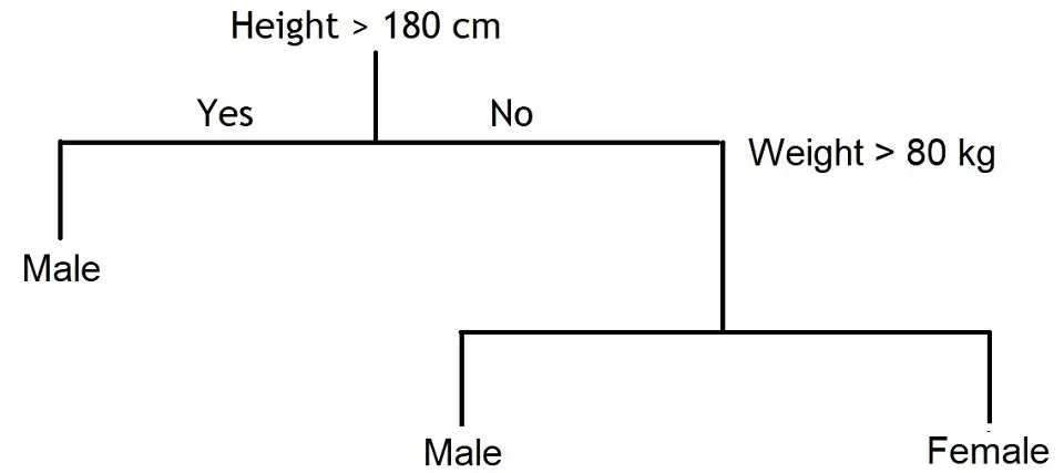
The process of building a Classification Decision tree is through an iterative process of splitting the data into partitions and then splitting it again on each node. 

A visual example of a classification tree is shown below. 

Regression Trees

The target variable can take continuous values in regression trees, typically real numbers. 

Continuous variables are numeric variables that can also be a date or time, with infinite values between any two. An example of a continuous variable is the price of a house. 

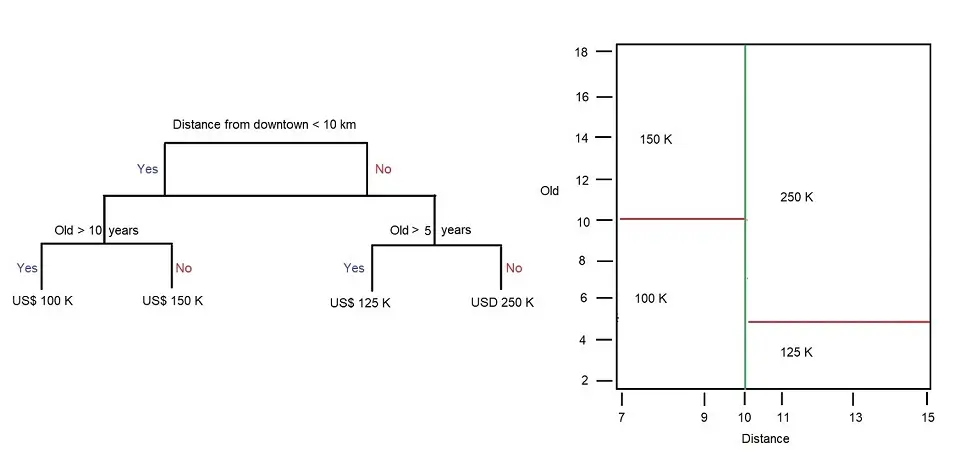
A visual example of a regression tree is shown below. For example, the regression tree below uses continuous variables: 

1. Houses far from the downtown area are less expensive
2. Old buildings/apartments/houses are less expensive

The root node in this example is ‘Distance from downtown <10km’, and the internal node is how old the building/apartment is, in this example, ‘Old > 10 years’ and ‘Old > 5 years’.

Below are two different representations of a small Regression tree. We have the Regression Tree on the left, allowing us to explore the Root and internal nodes, and on the right, we have how the space is partitioned. The blue line represents the first partitioning of the tree, and the red lines represent the following partitions. The numbers at the end of the tree and in the partitions represent the value of the response variable.

For example, houses/apartments/buildings with a distance > 10km from downtown and are older than 10 years are more expensive. A house 11km away from downtown that is 4 years old will be roughly 125k, whereas if the house were 16 years old, it would be in the 250k price range.

What is the difference between a Classification and a Regression tree? 

A Classification tree splits the data set based on the similarity of the data. For example, two variables, income, and age, can be used to determine whether or not a consumer will buy a particular brand or model of phone.

If the training data output indicates that 95% of people over 30 bought a particular phone, the data gets split there, and age becomes a top node in the tree. This split allows us to interpret that the data is “95% pure”. Further analysis using measures of impurity such as entropy or Gini index is used to measure the homogeneity of the data when it comes to classification trees.

In a Regression tree, the model is fit to the target variable, which can take continuous values. Using each independent variable, the data then splits at several points for each independent variable. The error between predicted and actual values is squared at each split to get “A Sum of Squared Errors” (SSE). The SSE is compared to the other variables, and the variable with the lowest SSE is chosen as the split point. This process is continued recursively.

Different algorithms choose the features and also determine when to stop the process of splitting based on the kind of tree that is being built. There are various trees, but the two main ones that we will discuss are CART and ID3.

Classification and Regression Trees (CART)

Classification and regression decision trees are collectively called CART (Classification and Regression Trees)

These trees use an index called the Gini Index to determine which features to use and the order of the features in the process of splitting. It is calculated for each feature by subtracting the sum of the squared probabilities of each target class from 1.

In the above formula, p is the probability. The lower the Gini Index, the higher the homogeneity. Therefore, the feature with the lower Gini index is chosen. Let’s take the case of the students playing the piano and calculate the Gini index.

Gini Index for Gender:

• Gini for sub-node Female = (0.2)*(0.2)+(0.8)*(0.8)=0.68
• Gini for sub-node Male = (0.65)*(0.65)+(0.35)*(0.35)=0.55
• Weighted Gini for split Gender = (10/30)*0.68+(20/30)*0.55 = 0.59

Gini Index for Play Other Instruments:

• Gini for sub-node Yes= (0.42)*(0.42)+(0.58)*(0.58)=0.51
• Gini for sub-node No= (0.56)*(0.56)+(0.44)*(0.44)=0.51
• Weighted Gini for split Play Other Instruments= (12/30)*0.51+(18/30)*0.51 = 0.51

The Gini Index for Class:

• Gini for sub-node 8th Grade= (0.43)*(0.43)+(0.57)*(0.57)=0.51
• Gini for sub-node 9th Grade= (0.56)*(0.56)+(0.44)*(0.44)=0.51
• Weighted Gini for split Class = (14/30)*0.51+(16/30)*0.51 = 0.51

Based on the above Gini Indices, the Decision Tree will split on either Plays Other Instruments or Class, depending on which Index is lower when more decimal points are considered.

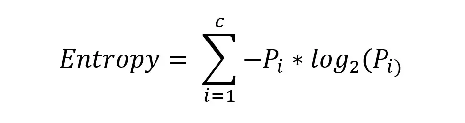
ID3 (Iterative Dichotomiser 3)

This type of tree uses a value called Information Gain or Entropy to determine which features to use. Information Gain multiplies the probability of the class times the log (base=2) of that class probability.

Everything mentioned above might seem a little complicated, but there are Python libraries that make using this algorithm super easy! All you need to do is write three lines of code, and everything I’ve explained so far happens behind the scenes.

First, we import the Decision Tree Classifier from the Scikit-Learn Tree library.

from sklearn.tree import DecisionTreeClassifier

Then, we create the model and fit it into the data

dt = DecisionTreeClassifier()
dt.fit(X, y)

And that’s it! The tree has now been fitted on the data, which basically means a decision tree has been created based on the data you provided to the algorithm. Now, you can give the tree some new data that doesn’t have corresponding labels and ask it to predict them.

dt.predict(test)

Pros and Cons of Decision Trees

Pros of Decision Trees:

1. Simplicity: Trees can be visualized, making it easier to understand and interpret the results. 

2. Numeric and Categorical Data – Decision trees can handle both numerical and categorical data

3. Little Data Preparation: Other techniques may require more work, such as data normalization, blank values, and the creation of dummy variables. 

4. White box model: For a model to be considered a white box, it must be understandable, and the Machine Learning process must be transparent. In decision trees, the results can be easily derived by boolean logic. 

5. Multiple outputs: A decision tree can handle multiple output problems, giving more insight and understanding to make better decisions. 

6. Validate the model: You can validate a model using statistical tests such as accuracy. This helps to understand the model’s reliability and how reliant one can be to make decisions on it. 

Cons of Decision Trees:

1. Overfitting: Due to decision trees’ ability to create complex trees, there is a possibility of overfitting. Overfitting is a modeling error when a function is too closely fit to a limited set of data points. To avoid this, you can use pruning, for example, setting a maximum on the depth of the tree. 

2. Unstable: A small change in the data can lead to a significant overall change in the structure of the optimal decision tree, leading to completely different trees being generated. 

3. Inaccuracy: There are other predictors which perform better with similar data sets. You can choose to use a random forest instead of a decision tree. However, a random forest is not as easy to understand and interpret. 

Concept of Bias and Variance

Bias and Variance are two concepts associated with decision trees (and machine learning algorithms in general, too), and if either one is high, then the algorithm isn’t efficient enough.

Bias: This is the average difference between predicted and actual values.

Variance: This is the difference in predictions if different samples are taken from the same population.

A balance between the two must be found, and the techniques that perform a trade-off management analysis between bias and Variance come under “ensemble learning.”

Ensemble Learning Techniques

1. Bagging

This process involves:

• breaking the main data set into smaller subsets of data,
• fitting a classifier on each subset, and so having multiple classifiers and
• combining the predictions of each classifier using mean/median/mode.

2. Boosting

This process forms a strong classifier from several weak classifiers sequentially.

There are many applications of Decision trees in real life, such as Biomedical Engineering, in which they use them to identify features for implantable devices. It is also used in Sales and Financial analysis, which helps customer satisfaction regarding a product or service.