Data Visualization Using Python

We have seen that Python language is a powerful tool for data science and data operations, but how powerful is Python for Data visualization?

One of the key responsibilities of Data scientists is to communicate results effectively with the stakeholders. This is where the power of visualization comes into play. Creating effective visualizations helps businesses identify patterns and subsequently helps in decision-making.

Importance of Data Visualization

It is essential for a data scientist as well to visualize data first. Data visualization is extracting information about data using various visualization techniques. It helps develop a deep understanding of the data before moving to the next step of training machine learning models.

Imagine you have a giant puzzle, where each piece is a tiny bit of data. Each piece alone might not tell you much, but put them together correctly, and a clear picture emerges! Data visualization does this for data science and operations – it puts all those tiny bits of data together to show us a clear and complete picture.

In the world of data science, visualizing data is like creating a map that helps scientists find patterns, spot problems, and tell a story about the data to others. It turns rows of numbers into images that can quickly tell us what’s happening. It’s very important because it helps in understanding the data easily.

In data operations, having good visuals, like charts or graphs, helps people see how well their systems work. It’s like having a dashboard in a car where you can quickly see if you’re running out of gas or if the engine is too hot. This way, they can quickly see and fix problems, ensuring everything runs smoothly.

Python, a popular programming language, gives us many tools to create these helpful visuals. With Python, you can make simple graphs, fancy charts, or even interactive maps that help us understand our data better. This article will discuss using Python to turn our data into informative visuals with tutorials.

Tools for this Visualization Tutorial

I will explain various plots using a popular Seaborn library for Python data visualization. Seaborn is a library that provides advanced visualizations compared to “matplotlib.”

In this article, I will be using the example dataset from the Kaggle competition. You may also look at the code in this HTML file, and in case you wish to execute the code while going through this article, you may check out the Jupyter file for Data Visualization using Pandas in Python.

So, now let’s see the steps for Data visualization using Python. These are as follows:

1. Importing Python Packages for Visualization

The first step before doing anything is to import packages used to create the visualizations.

import pandas as pd
import matplotlib.pyplot as plt
import seaborn as sns
import numpy as np

2. Reading Dataset

After importing the data, the next step is to load the CSV file to the pandas’ dataset.

housePropertyDataset = pd.read_csv('house_property_sales.csv')

3. Seaborn Library

There is a seaborn library available to generate detailed chart representation.

sns.set()
 
plt.plot(housePropertyDataset['SalePrice'])

plt.legend(loc='upper right')
plt.show()

Chart Output

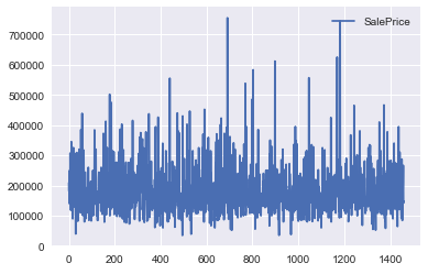
In the above example, we used the legend to display it and positioned it top-right.

4. Generating Visualization in Python

We can generate visualizations once data is imported into the panda’s data frame. There are diverse types of visualizations that we can generate from the dataset. Here we will be focusing on:

1. Zoom Axes
2. Generating Subplots
3. Box Plot
4. Two Dimension Histogram
5. Linear Regression Plots
6. Mesh grid
7. Strip Plot
8. Swarn Plot
9. ECDF Plot
10. Violin Plot
11. Joint Plot
12. Heatmap Plot
13. Pair Plot

Let’s get started:

Zoom Axes

We will now create the same figure as created in the Seaborn Library introduction. But setting the axis extends this time using “plt.xlim()” and “plt.ylim()“. These commands zoom, expand the plot, or set the axis ranges to include important values (such as the origin). Please check the Python code below:

sns.set()

# We can use the styles for the plot
# print(plt.style.available) used to print all available styles plt.style.use('ggplot')

plt.plot(housePropertyDataset['SalePrice'])

plt.xlabel('Property ID') plt.ylabel('Sales Price')
plt.xlim(1100,1200) plt.ylim(100000,800000)

plt.title('Price of various property located')

plt.show()

Visual Output

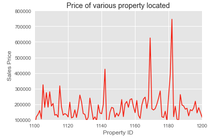
NOTE: After creating the plot, we can use “plt.savefig()” to export the image produced to a file.

Generating Subplots

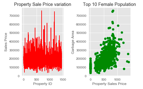
Using subplots is a better alternative than using “plt.axes()”. This is because we can manually add multiple plots in the same figure.

The subplot accepts three arguments,

subplot(n_rows, n_columns, n_subplot)

Subplot ordering is row-wise, starting from the top left corner. The Python code for the same is as follows:

plt.style.use('ggplot')

plt.subplot(1,2,1)
plt.plot(housePropertyDataset['SalePrice'], color='red') plt.title('Property Sale Price variation')
plt.xlabel('Property ID')
plt.ylabel('Sales Price')

plt.subplot(1,2,2) plt.scatter(housePropertyDataset['GarageArea'],housePropertyDataset['SalePrice'], color='green')
plt.title('Top 10 Female Population')
plt.xlabel('Property Sales Price')
plt.ylabel('Garbage Area')

# Improve the spacing between subplots and display them plt.tight_layout()
plt.show()

Output Using Subplots

Box Plot

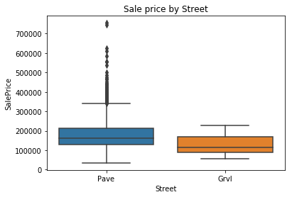
Boxplot is an important EDA plot that helps to understand data precisely. When we plot a box plot, it gives the following details:

1. Outliers: These are the extreme values in the dataset. We need to choose whether these outliers are required in the dataset or if we can remove them for accurate results.
2. Inter Quartile Range (IQR): It is the difference between the upper quartile (75th percentile) and the lower quartile (25th percentile).
3. 75th Percentile: It is the 75th percentile of the dataset.
4. 50th Percentile: It is the 50th percentile of the dataset. They are also called Median.
5. 25th Percentile: It is the 25th percentile of the dataset.
6. The extent of data: The whisker extends to the 1.5 IQR of the extreme of the data, whichever is less extreme.

Consider the example shown below:

sns.boxplot(x='Street', y='SalePrice', data=housePropertyDataset) plt.title('Sale price by Street')
plt.show()

Output with Box Plot

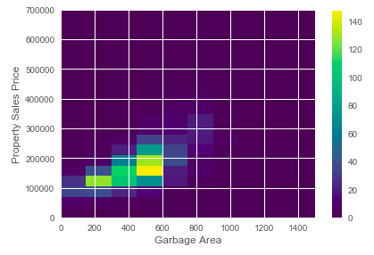
Two Dimension Histogram

We can also generate a 2-D histogram using a “hist2D” function of Python. Let’s look at an example shown below:

x = housePropertyDataset['GarageArea']
y = housePropertyDataset['SalePrice']
plt.hist2d(x,y, bins=(10,20), range=((0, 1500), (0, 700000)), cmap='viridis')

plt.colorbar()

plt.xlabel('Garbage Area')
plt.ylabel('Property Sales Price')

plt.tight_layout()
plt.show()

2-D Histogram Output:

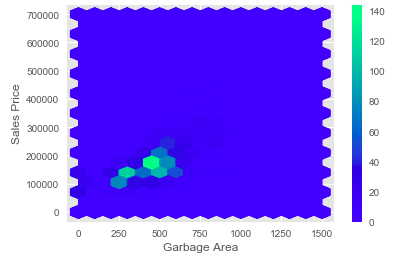
Hexagonal Bins Visualization

As shown above, we have created rectangular bins for a 2D array. Similarly, we can also generate hexagonal bins as well in Python.

x = housePropertyDataset['GarageArea']
y = housePropertyDataset['SalePrice']
plt.hexbin(x,y, gridsize=(15,10),extent=(0, 1500, 0, 700000), cmap='winter')

plt.colorbar()

plt.xlabel('Garbage Area')
plt.ylabel('Sales Price')
plt.show()

Hexagonal Bin Visual Output

Linear Regression Plots

We can generate a regression plot using the seaborn library. Seaborn provides “lmplot()” function to generate regression plots.

# Plot a linear regression between 'GarageArea' and 'SalePrice' sns.lmplot(x='GarageArea', y='SalePrice', data=housePropertyDataset,
col='Street') # We can also use 'hue' parameter instead of col parameter to plt on the same graph
# Display the plot
plt.show()

Regression Plot Output

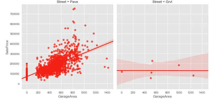
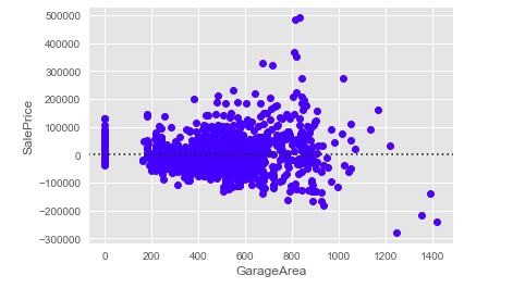
Residual Plot

As we can see from the above plot, all points are not passing through the straight line. Therefore, we have residuals in the plot (or, in other terms, deviation in data from the plotted line). Seaborn provides “residplot()” function using which we can generate residual plot:

sns.residplot(x='GarageArea', y='SalePrice', data=housePropertyDataset, color='blue')
# Display the plot
plt.show()

Residual Plot Output

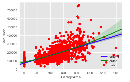
Plotting Second-Order Regression Plots

It is also possible to generate higher-order regression plots using order argument in “regplot” function provided by the seaborn library.

plt.scatter(housePropertyDataset['GarageArea'],housePropertyDataset['SalePrice'], label='data', color='red', marker='o')

sns.regplot(x='GarageArea', y='SalePrice', data=housePropertyDataset , scatter=None, color='blue', label='order 1', order=1)

sns.regplot(x='GarageArea', y='SalePrice', data=housePropertyDataset , scatter=None, color='green', label='order 2', order=2)

plt.legend(loc='lower right')
plt.show()

Second Order Regression Plot Output

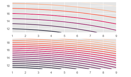
Mesh Grid

Mesh grid transforms the domain specified by vectors x and y into arrays X and Y, which can be used to evaluate the functions of two variables.

In the example below, we use the formula 3 * sqrt(x^2 + y^2).

u = list(range(1, 10))
v = list(range(11, 20))
X,Y = np.meshgrid(u,v)
Z = 3*np.sqrt(X**2 + Y**2)

plt.subplot(2,1,1)
plt.contour(X, Y, Z)

plt.subplot(2,1,2)
plt.contour(X, Y, Z, 20) # 20 contour

plt.show()

Mesh Grid Output

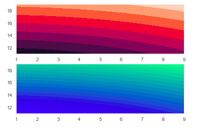
As we have seen above, the “contour” function generates lines, but to have the lines with colors, we can use a “contourf()” function.

u = list(range(1, 10))
v = list(range(11, 20))
X,Y = np.meshgrid(u,v)
Z = 3*np.sqrt(X**2 + Y**2)

plt.subplot(2,1,1)
plt.contourf(X, Y, Z)

plt.subplot(2,1,2)
plt.contourf(X, Y, Z, 20, cmap='winter') # 20 contour will be mapped

plt.show()

Mesh Grid Outpur with Colors

Strip Plot

Seaborn provides “stripplot()” function, which allows us to visualize data categorically. Refer to the example shown below:

plt.subplot(1,2,1)
sns.stripplot(x='Street', y='SalePrice', data=housePropertyDataset, jitter=True, size=3)
plt.xticks(rotation=90)

plt.subplot(1,2,2)
sns.stripplot(x='Neighborhood', y='SalePrice', data=housePropertyDataset, jitter=True, size=3)
plt.xticks(rotation=90)

plt.subplots_adjust(right=3)
plt.show()

Strip Plot Output

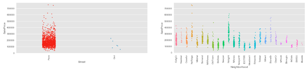
NOTE: In the example shown above, we have used “jitter” flag to avoid overlapping of the same data points.

Swarn Plot

When we plot data using the histogram, curves look different based on the bins chosen. So, it may confer different results based on the bins chosen. To overcome biased results from the histogram, the “swarn” plot is recommended.

plt.subplot(1,2,1)
sns.swarmplot(x='Street', y='SalePrice', data=housePropertyDataset, hue='SaleCondition')
plt.xticks(rotation=90)

plt.subplot(2,2,2)
sns.stripplot(x='Neighborhood', y='SalePrice', data=housePropertyDataset, hue='SaleCondition')
plt.xticks(rotation=90)

plt.subplots_adjust(right=3)
plt.show()

Swarn Plot Output

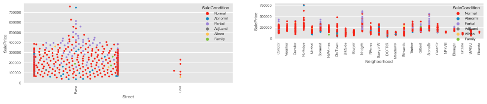
The Strip plot is also a great way to visualize data. However, the data points tend to overlap when we have massive data. An alternative is to use a “swarn” plot where data points don’t overlap each other.

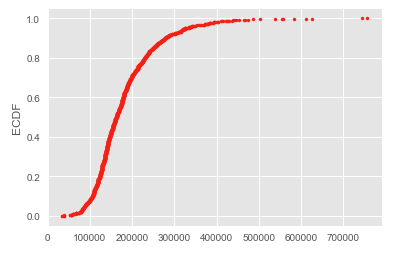
ECDF Plot

At times, when we have a vast amount of data, the data points overlap in the “swarn” plot. The “swarn” plot doesn’t give a precise result to study in such a scenario. It is recommended to use ECDF (Empirical Cumulative Distribution Function).

The x-axis has sorted data, and the y-axis has evenly spaced data points.

def ecdf(data):
 # Number of data points: n
 n = len(data)
 # x-data for the ECDF: x
 x = np.sort(data)
 # y-data for the ECDF: y
 y = np.arange(1, n+1) / n 
 return x, y

SalePrice = housePropertyDataset['SalePrice'] x_vers, y_vers = ecdf(SalePrice)

plt.plot(x_vers, y_vers, marker = '.', linestyle = 'none')

plt.ylabel('ECDF')

plt.show()

ECDF Plot Output

Violin Plot

Violin Plots are like a box plot. They also show the max, min, and median of the dataset. In the Violin plot, the distribution is denser, whereas the plot is thicker. Check the following Python code:

plt.subplot(2,1,1)
sns.violinplot(x='SaleType', y='SalePrice', data=housePropertyDataset)

plt.subplot(2,1,2)
sns.violinplot(x='SaleType', y='SalePrice', data=housePropertyDataset, color='lightgray', inner=None)

sns.stripplot(x='SaleType', y='SalePrice', data=housePropertyDataset, jitter=True, size=1.5)

plt.show()

Violin Plot Output

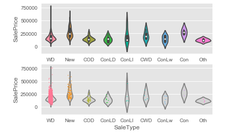
NOTE: We can also generate a combined plot. The second plot combines the Strip and Violin plots in the example above.

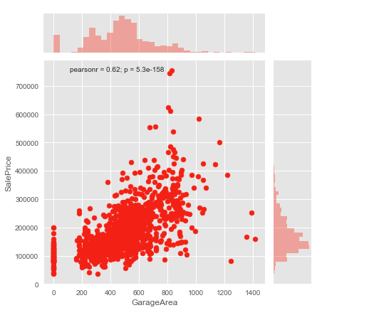
Joint Plot

The joint plot shows how the data varies on the x-axis when there is a change in the y-axis. The Joint plot also computes the Pearson coefficient and the p-value. I will explain the Pearson coefficient and p-value more in the upcoming post.

fig = plt.figure(figsize = (16,89))
sns.jointplot(x='GarageArea', y='SalePrice', data=housePropertyDataset)
plt.xticks(rotation=90)
plt.show()

Joint Plot Output

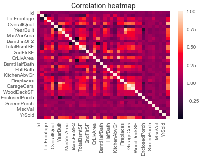
Heatmaps

A heatmap plot is useful for determining how the feature depends on the other. 

In the example below, we plotted a Correlation heatmap of the dataset’s features. We can see that lighter colors depict a positive correlation. Check the code:

numeric_features = housePropertyDataset.select_dtypes(include=[np.number])
sns.heatmap(numeric_features.corr())
plt.title('Correlation heatmap')
plt.show()

Heatmap Output

Pair Plot Visualization in Python

It is the plot using which we can quickly glimpse the data. Here, we can plot the possible combination of our dataset’s features(columns). Consider an example shown below:

data = housePropertyDataset[['SaleCondition', 'SalePrice','OverallQual', 'TotalBsmtSF','GrLivArea','GarageArea','FullBath','YearBuilt','YearRemodAdd']]
sns.pairplot(data, hue='SaleCondition')
plt.show()

Pair Plt Output

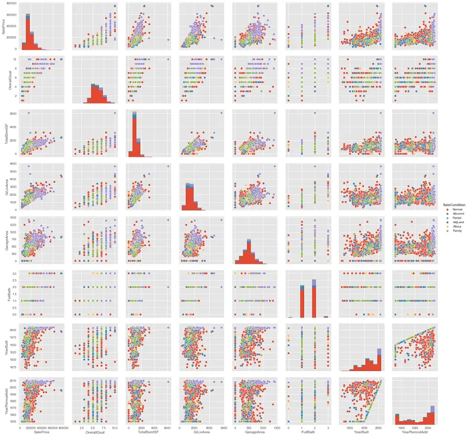
NOTE: Using a pair plot, we can only plot numeric columns of the dataset.

In this post, we have seen the advantages of using the Seaborn library and the “matplotlib” library. However, the Seaborn Library offers much more advanced visualizations, which can help us understand our dataset.

I hope you now have some data visualization techniques using Python for your next project or to discuss with the business stakeholders.