How to Analyze High-Dimensional Data in Machine Learning

Before we discuss analyzing high-dimensional data for machine learning, let’s see what high-dimensional data is and its importance.

What is High-Dimensional Data?

High-dimensional data refers to datasets with many features (variables or attributes) relative to the number of observations (samples or instances). More straightforwardly, it’s data that has many columns and potentially fewer rows. Each feature represents a dimension in the data space. As the number of features increases, so does the dimensionality of the data.

Characteristics of High-Dimensional Data:

1. Large Feature Set:
   • Numerous variables or attributes.
   • Potentially having more features than observations (p >> n, where p = number of features and n = number of observations).
2. Sparsity:
   • Many features might have a majority of zero or missing values.
   • Some dimensions may not add significant information.
3. Complexity:
   • Higher difficulty in visualizing, understanding, and interpreting data.
   • Increased computational complexity and processing time.

Challenges with High-Dimensional Data:

1. Curse of Dimensionality:
   • As dimensions increase, the volume of the space increases exponentially, making the available data sparse.
   • Distance measures become less meaningful due to the increased space, diminishing the performance of models based on distance (like k-Nearest Neighbors).
2. Overfitting:
   • Models can easily overfit the training data, capturing noise instead of underlying patterns, which hampers generalization to new data.
3. Computational Burden:
   • Processing high-dimensional data requires more computational resources and time.
   • Efficient storage and handling of data become pivotal.
4. Model Interpretability:
   • With more features, models become complex and hard to interpret or explain.
   • It’s challenging to understand the influence and interaction of each feature in predictions.

Handling and Analyzing High-Dimensional Data:

1. Dimensionality Reduction:
   • Techniques like Principal Component Analysis (PCA), t-distributed Stochastic Neighbor Embedding (t-SNE), and autoencoders can reduce the dimensionality while preserving as much information as possible.
2. Feature Selection:
   • Identify and utilize a subset of the most informative features.
   • Techniques include wrapper methods, filter methods, and embedded methods.
3. Regularization:
   • In model training, employ regularization methods (like Lasso, Ridge, or Elastic Net) to prevent overfitting and handle high-dimensional data effectively.
4. Sampling Techniques:
   • Use methods like Random Under-Sampling (RUS) or Random Over-Sampling (ROS) to handle imbalances in the data.

Applications of High-Dimensional Data:

• Bioinformatics: Analyzing gene expression data.
• Image Processing: Handling pixel values in image data.
• Financial Forecasting: Analyzing numerous financial indicators.
• Text Analysis: Working with a large vocabulary in text data.

While high-dimensional data can capture detailed and complex structures, efficiently managing and extracting meaningful patterns from such data demands specialized techniques and careful consideration of the associated challenges.

Importance of Analyzing High-Dimensional Data in ML

Analyzing high-dimensional data in machine learning (ML) is crucial for various reasons, especially as numerous real-world problems involve dealing with such data. High-dimensional data refers to datasets with many features (or variables) relative to the number of observations. Here are some key points concerning the importance of handling and analyzing high-dimensional data in ML:

1. Revealing Hidden Patterns

• Uncovering Insights: High-dimensional data can encapsulate rich, intricate patterns that may remain concealed in lower-dimensional representations.
• Feature Interactions: Analyzing numerous features allows machine learning models to explore potential interactions and dependencies, which could be pivotal for making accurate predictions.

2. Enhancing Predictive Performance

• Better Modeling: More features might enable a model to capture underlying complexities and thus improve predictive performance, given that the model and methodology are aptly chosen.
• Diverse Applications: High-dimensional data analysis is indispensable in various domains like genomics, finance, and image analysis, where datasets inherently possess many features.

3. Facilitating Personalization

• Customer Segmentation: High-dimensional data in marketing and e-commerce allows for detailed customer segmentation and targeted marketing by analyzing customer characteristics and behaviors.
• Recommendation Systems: In building recommendation systems, models leverage high-dimensional user-item interaction data to deliver personalized content or product suggestions.

4. Navigating Challenges

• Curse of Dimensionality: Although high-dimensional data can be advantageous, it introduces the “curse of dimensionality,” where models face challenges due to the vastness of the feature space. Effective analysis methods are essential to navigate through these challenges.
• Feature Selection: Analyzing high-dimensional data necessitates effective feature selection and dimensionality reduction techniques to extract meaningful information and mitigate the risk of overfitting.

5. Enabling Complex Models

• Deep Learning: High-dimensional data is particularly pivotal for training deep learning models, which can manage numerous input features and automatically discern relevant feature interactions.
• Enhanced Capabilities: With a plethora of features, ML models can be enabled to learn and generalize better from complex datasets, solving intricate problems across various domains.

6. Advancing Scientific Research

• Biological Data Analysis: Genomic and proteomic data typically have a high-dimensional character, and analyzing this data is vital for advancing research in areas like disease prediction and drug discovery.
• Social Sciences: In social science research, analyzing high-dimensional data, such as social networks and communication patterns, helps understand social phenomena and behaviors.

7. Ensuring Robustness

• Diversity: High-dimensional data provides diverse features that could help models be more robust and generalize to unseen data.
• Avoiding Bias: By considering a wide array of features, models may avoid potential biases when focusing only on a limited set of predictors.

8. Informing Decision-Making

• Strategic Insights: For decision-makers, models utilizing high-dimensional data can provide comprehensive insights, aiding in more informed, strategic decisions.
• Risk Management: In sectors like finance and healthcare, analyzing high-dimensional data allows for better risk management by considering numerous variables and scenarios.

In summary, while high-dimensional data offers rich insights and enables the creation of sophisticated ML models, it also presents challenges that necessitate careful handling and analysis. Employing robust algorithms and integrating dimensionality reduction and feature selection strategies are pivotal in effectively leveraging high-dimensional data in ML applications.

It is impossible to draw images with more than three dimensions on paper. We can only draw visualizations in two dimensions (x-axis and y-axis) or, at the most, three dimensions (x-axis, y-axis, and z-axis), but without the ability to measure all those dimensions.

Similarly, let’s consider a dataset with 1000 features or dimensions. Visualizing the data on paper is impossible, and it is often even computationally challenging to train the Machine Learning models. So, we can reduce the data to one, two, or lower dimensions. Let’s look at multiple techniques for dimensionality reduction for the given dataset.

Techniques to Analyze High-Dimensional Data

Now that we have understood the concept of high-dimensional data and its importance, let’s discuss the techniques to analyze high-dimensional data in machine learning. These techniques are as follows:

Dimension Reduction using PCA

PCA stands for Principal Component Analysis.

As the name suggests, PCA is about the principal components of a multi-dimensional dataset. Not each of the components is significant and hence can be ignored. The principal components technique of the analysis identifies and computes the principal components and uses them as the base for the overall data change.

Principal Component Analysis (PCA) takes up data of several dimensions and flattens it to 2- or 3-dimensional space without loss of information. For example, think of a movie camera that fattens the 3-D image to a 2D image without much loss of information.

PCA de-correlates the measurements, plots the uncorrelated points, and measures their Pearson correlation. To find the PCA in using Python for data science, refer to the code shown below:

from sklearn.decomposition import PCA
from scipy.stats import pearsonr
from sklearn.datasets import load_wine

data = load_wine()
X = data.data
y = data.target

# No of features in the datset
print(len(data.feature_names))

model = PCA()

pca_features = model.fit_transform(X)

# 1st Feature/Dimension
xs = pca_features[:,0]

# 2nd Feature/Dimension
ys = pca_features[:,1]

correlation, pvalue = pearsonr(xs, ys)
print(correlation, pvalue)

Using PCA, we have generated features that contain the dataset’s information. Moreover, using two features, we can depict the same information in our dataset with all the features.

Using the PCA function provided by scitit-learn library, we have generated PCA features. However, we are also interested in knowing the variance of each PCA feature.

This is where the Intrinsic dimension comes in. The intrinsic dimension is the number of features to approximate the dataset. The intrinsic dimension is the number of PCA features with significant variance. It is a crucial step as low variance features add noise to the dataset.

We can generate a plot to determine each Principal Component’s variance. Please refer to the following code to generate a plot:

from sklearn.decomposition import PCA
from sklearn.preprocessing import StandardScaler
from sklearn.pipeline import make_pipeline
import matplotlib.pyplot as plt
from sklearn.datasets import load_wine

data = load_wine()
X = data.data
y = data.target

scaler = StandardScaler()
pca = PCA()

pipeline = make_pipeline(scaler, pca)

pipeline.fit(X)

print(pca.explained_variance_ratio_)

features = range(pca.n_components_)
plt.bar(features, pca.explained_variance_)
plt.xlabel('PCA feature')
plt.ylabel('Variance')
plt.xticks(features)
plt.show()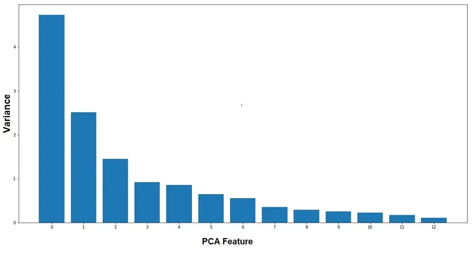

Observations:

1. In the above example, we use “StandardScaler” to scale the data.
2. PCA provides “n_components_“, which is of the same length as none of the feature dataset has.
3. PCA also provides “explained_variance_“, which depicts the variance of each feature.
4. After the 2nd PCA feature, the variance started decreasing gradually.
5. Additional PCA provides “explained_variance_ratio_“, using which we can observe that the first three feature covers 66% of the variance.

Our end goal is to reduce the number of features from the dataset. And we should reduce dataset dimensions to the number from which variance starts decreasing gradually.

Let us look at one more example using PCA for dimensionality reduction. In the example shown below, we reduce features to 3. (Specifying as a “n_components” argument to PCA function.) A good choice is to use the intrinsic dimension here. Please refer to the following code:

from sklearn.decomposition import PCA

pca = PCA(n_components=3)
pca.fit(X)
pca_features = pca.transform(X)

print(pca_features.shape)

plt.scatter(pca_features[:,0], pca_features[:,1], c=y)
plt.xlabel('First principal Component')
plt.ylabel('Second principal Component')
plt.show()

Output:

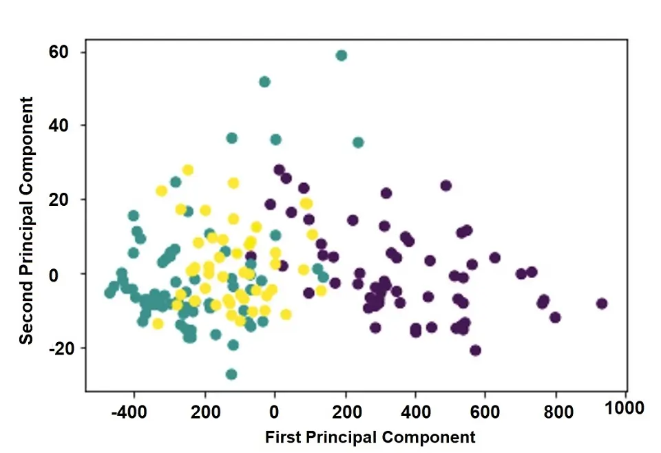
The above logic will take three features with high variance. We have successfully reduced the high-dimensional data set to 3 dimensions without losing much information.

t-Distributed Stochastic Neighbor Embedding (t-SNE)

t-SNE is also the dimension reduction technique. t-SNE takes up the high dimensional dataset (where we have a lot of features) and reduces it to a 2-D graph that retains a lot of original information.

The significant differences between t-SNE and PCA are:

1. PCA is the linear feature extraction technique, whereas t-SNE is a non-linear feature extraction technique suited for high-dimensional data.
2. t-SNE is computationally expensive and can take much time on large datasets where PCA will finish in seconds or minutes.
3. t-SNE is the probabilistic technique, whereas PCA is a mathematical technique.

Let’s look at an example of the code showing how to perform the t-SNE algorithm on a dataset with huge features:

from sklearn.manifold import TSNE

tsne_features = TSNE().fit_transform(X)

plt.scatter(tsne_features[:,0], tsne_features[:,1], c=y)
plt.xlabel('First t-SNE Feature')
plt.ylabel('Second t-SNE Feature')
plt.show()

NOTE: 

1. t-SNE only has a fit_transform method. It has no separate fit and transforms processes.
2. If the dataset has many features, it’s good practice to reduce the noise using PCA (maybe to 50 features) and then apply t-SNE. (As t-SNE is an expensive operation).

Dimension Reduction on CSR Matrix

Let’s say we are analyzing documents with written content. In this case, the “word frequency array” Word frequency array represents the frequency of the word in each document. The rows of the array represent the documents, and the columns of the array represent the frequency of the words in the documents.

For example, consider that we have a sample of two documents. In the first document, the words are “love,” “dimensionality,” “reduction,” and “dimensionality.” In the second document, we have the words “dimensionality,” “reduction,” “CSR,” and “Matrix.” The word frequency array of the above two documents will be as shown in the table below:

Document	Love	Dimensionality	Reduction	CSR	Matrix
#1	1	2	1	0	0
#2	0	2	1	1	1

In the table above, the rows represent different documents, and the column represents the unique words for all the documents.

NOTE: The above representation is very naive as it depends only on the frequency of the words. There is a better representation called TF-IDF representation, where TF stands for Term Frequency and IDF stands for Inverse Document Frequency.

It is self-explanatory when we look at the above-mentioned “word frequency table” that if the words in the document are different, there will be many columns where the word frequency will be zero for the given document. 

Sparse Array

An array where most entries are zero is known as a Sparse array. We can represent the sparse array using CSR Matrix instead of a NumPy matrix, as CSR matrix typically saves space on the storage drive.

We cannot apply PCA on CSR Matrix. In such a case, we need to use “TruncatedSVD” function for dimension reduction.

Consider an example of the code shown below:

from sklearn.feature_extraction.text import TfidfVectorizer
from sklearn.decomposition import TruncatedSVD
from sklearn.cluster import KMeans
from sklearn.pipeline import make_pipeline
import pandas as pd
import requests
from bs4 import BeautifulSoup

# Preparing document
html = requests.get('https://en.wikipedia.org/wiki/Sundar_Pichai')
soup = BeautifulSoup(html.text, 'lxml')
document = []

text = [''.join(t.findAll(text = True)) for t in soup.findAll('h2')]

# Generating CSR Matrix
tfidf = TfidfVectorizer()
csr_mat = tfidf.fit_transform(documents)

words = tfidf.get_feature_names()
print(words)

# Performing Dimension Reduction
svd = TruncatedSVD(n_components=50) kmeans = KMeans(n_clusters=6) pipeline = make_pipeline(svd, kmeans)

pipeline.fit(csr_mat)
labels = pipeline.predict(csr_mat)

df = pd.DataFrame({'label': labels, 'article': text}) print(df.sort_values('label'))

Here in the example above:

1. We are generating a document using a Wikipedia page.
2. We use TfidfVectorizer, which transforms a list of documents into a word frequency array, which it outputs as a csr_matrix.
3. Once CSR Matrix is generated, we are using “TruncatedSVD” function for dimension reduction.

Non-negative Matrix Factorization (NMF)

NMF is also the dimension reduction technique. One needs to use NMF typically when text is involved. To use NMF, all the sample data should be non-negative. It works with NumPy array and CSR Matrix as well.

Refer to the sample code shown below to use the NMF technique:

from sklearn.decomposition import NMF
import pandas as pd
import requests
from bs4 import BeautifulSoup
import numpy as np
from sklearn.feature_extraction.text import TfidfVectorizer

# Preparing Document
html = requests.get('https://en.wikipedia.org/wiki/Sundar_Pichai')
soup = BeautifulSoup(html.text, 'lxml')
text = [''.join(t.findAll(text = True)) for t in soup.findAll('h2')]

# Generating CSR Matrix
tfidf = TfidfVectorizer()
csr_mat = tfidf.fit_transform(text)

# Applying NMF
model = NMF(n_components=6)
model.fit(csr_mat)

nmf_features = model.transform(csr_mat)

df = pd.DataFrame(nmf_features, index=text)
print(df.head())

components_df = pd.DataFrame(model.components_, columns=words) component = components_df.iloc[3,:]
print(component.nlargest())

Unlike NMF, PCA doesn’t learn the parts of things. Its components do not correspond to topics (in the case of documents) or parts of images when trained on images.

Summary

In this article, we have talked about dimension-reduction techniques for analyzing high-dimensional data, including the following:

1. Principal Component Analysis (PCA) and intrinsic dimension.
2. t-SNE is used to reduce the dimensions of the high-dimensional dataset.
3. Dimension reduction on CSR Matrix. We saw how to generate a word frequency CSR matrix and apply dimension reduction techniques.
4. NMF dimension reduction technique, which is used for mostly text data.

I hope you have enjoyed this guide to analyzing high-dimensional data for machine learning. I know there is a lot to digest. Therefore, I recommend reading and implementing the learning/concepts.