A Guide to Gradient Descent in Machine Learning

In machine learning, optimizing the learning models is a critical step. This is where Gradient Descent emerges as a central optimizing algorithm.

What is Gradient Descent?

Machine learning hinges on creating models that predict outcomes from various inputs. However, these models don’t start perfectly; they initially operate on random parameters, which are not ideal for making accurate predictions.

Creating a machine learning model begins with defining what we want it to predict or decide based on a given set of inputs, known as features. These inputs might be anything from numbers in a spreadsheet to pixels in an image. The model looks at these inputs and tries to learn patterns that it can use for future predictions.

However, crafting a machine learning model is not just about feeding data and expecting accurate predictions immediately.

Initially, our models start with random guesses. They assign random values to what we call “parameters” or “‘”weights”. These assigned values of “weights” are essentially the factors the model considers when making its predictions.

At this early stage, the model’s predictions are likely to be inaccurate because it hasn’t yet learned the correct values for these parameters.

Gradient Descent steps in to address this challenge. It is an optimization algorithm that guides machine learning models from their initial, inaccurate state towards a more refined and accurate one.

By iteratively adjusting the model’s parameters against the direction of the gradient of the error function, Gradient Descent reduces the prediction errors, enhancing the model’s performance.

The effectiveness of Gradient Descent is in its handling of the ‘Cost Function’ or ‘Loss Function’. This function measures the discrepancy between the model’s predictions and the actual outcomes.

The primary goal of Gradient Descent in machine learning is to minimize this cost, thereby optimizing the model’s parameters for better predictions.

Understanding the Cost (Loss) Function in Machine Learning

In machine learning, the Cost Function, often interchangeably called the Loss Function, is a fundamental concept, especially in the optimization process undertaken by algorithms like Gradient Descent. This function is at the heart of model training and is crucial in guiding models towards more accurate predictions.

What is the Cost Function?

The Cost Function is a mathematical formula that measures the difference between the predicted output of a machine learning model and the actual output or the ground truth. It quantifies the model’s error, providing a numerical value that represents how well (or poorly) the model is performing.

This function is crucial because it gives us a concrete way to see how accurate our model is. Moreover, it provides a pathway to improve it.

Types of Cost Functions

There are several types of Cost Functions that we use in various machine learning models. These include the following:

• Mean Squared Error (MSE): Commonly used in regression problems. It calculates the square of the difference between the predicted and actual values and then averages these squared differences.
• Cross-Entropy: Often employed in classification tasks. It measures the performance of a classification model whose output is a probability value between 0 and 1.
• Hinge Loss: Used for ‘maximum-margin’ classification, most notably for support vector machines (SVMs).

Role of Cost Function in Gradient Descent

Gradient Descent is an optimization algorithm for minimizing the Cost Function. The algorithm iteratively adjusts the model’s parameters to find the combination of weights that results in the smallest possible value for the Cost Function.

In simpler terms, Gradient Descent navigates through the different possible values of the parameters to find those that lead to the least amount of error, as indicated by the Cost Function.

Why is the Cost Function Important?

1. Performance Indicator: It provides a clear metric to evaluate how well a model is performing.
2. Guide for Model Improvement: By minimizing the Cost Function, models can be fine-tuned to improve their accuracy.
3. Decision-Making for Parameter Adjustment: The Cost Function guides the direction and magnitude of adjustments in the model’s parameters during training.

In conclusion, the Cost Function is more than just a measure of error. It is a guiding light for machine learning models, helping them learn from their mistakes and improve over time. Understanding and appropriately selecting the right Cost Function is pivotal in machine learning, particularly when using algorithms like Gradient Descent for model optimization.

Understanding the Concept of a Gradient

A gradient in mathematics is often described as the slope of a curve at a particular point. This slope can vary depending on the direction in which it is measured. In the context of functions, a gradient provides vital information about the rate of change of the function’s output with respect to changes in its inputs.

When dealing with a function of a single variable (a univariate function), the gradient is simply the first derivative of that function. This derivative represents the rate of change of the function’s output relative to changes in its single input value.

In contrast, for functions of multiple variables (multivariate functions), the gradient is a vector. This gradient vector consists of the partial derivatives of the function with respect to each input variable. These partial derivatives collectively represent the function’s slope in each dimension of its input space.

An Example to Illustrate

Consider the function f(x) = 2x² + 3x. To understand the gradient of this function, we look at its first-order derivative with respect to x. The derivative, denoted as df(x)/dx, provides the rate at which f(x) changes as x changes.

For our function, the first-order derivative is calculated as follows: df(x)/dx = 4x + 3

This derivative tells us that for every unit increase in x, the output of the function f(x) changes by an amount equal to 4x + 3. This rate of change is what we refer to as the gradient in the univariate case.

Understanding the concept of a gradient is fundamental in various fields, including calculus and machine learning, especially when optimizing functions using techniques like Gradient Descent.

How Does Gradient Descent Work?

As mentioned earlier, Gradient Descent is a first-order iterative optimization algorithm that is central to many machine learning models. It aims to minimize a cost function by iteratively moving toward the steepest decrease in cost. The ‘steepness’ of the descent is determined by the first-order derivative—or the gradient—of the cost function with respect to the model’s parameters.

Here’s how it works:

1. Starting Point: The process begins with an initial guess for the model’s parameters, also known as ‘weights’. This starting point is typically random or based on some heuristic.
2. Computing the Gradient: The gradient of the cost function is computed at the current set of parameters. This gradient, which is a vector of partial derivatives, indicates the direction and rate of the steepest increase in cost.
3. Determining the Direction: The sign of each component of the gradient tells us the direction in which the corresponding parameter should be adjusted:
   • A positive gradient for a parameter suggests that increasing that parameter will increase the cost function, and thus, to decrease the cost, we should move in the negative direction.
   • Conversely, a negative gradient implies that decreasing the parameter will increase the cost, so we should move in the positive direction.
4. Updating Parameters: The parameters are then updated in the opposite direction of the gradient, scaled by a factor known as the ‘learning rate’. This step size is crucial as too large a step can overshoot the minimum, while too small a step can lead to a long convergence time.
5. Iterative Process: The steps of computing the gradient and updating the parameters are repeated until the changes in the cost function become negligibly small, indicating that the minimum cost has been approached.

Further Explanation About the Working

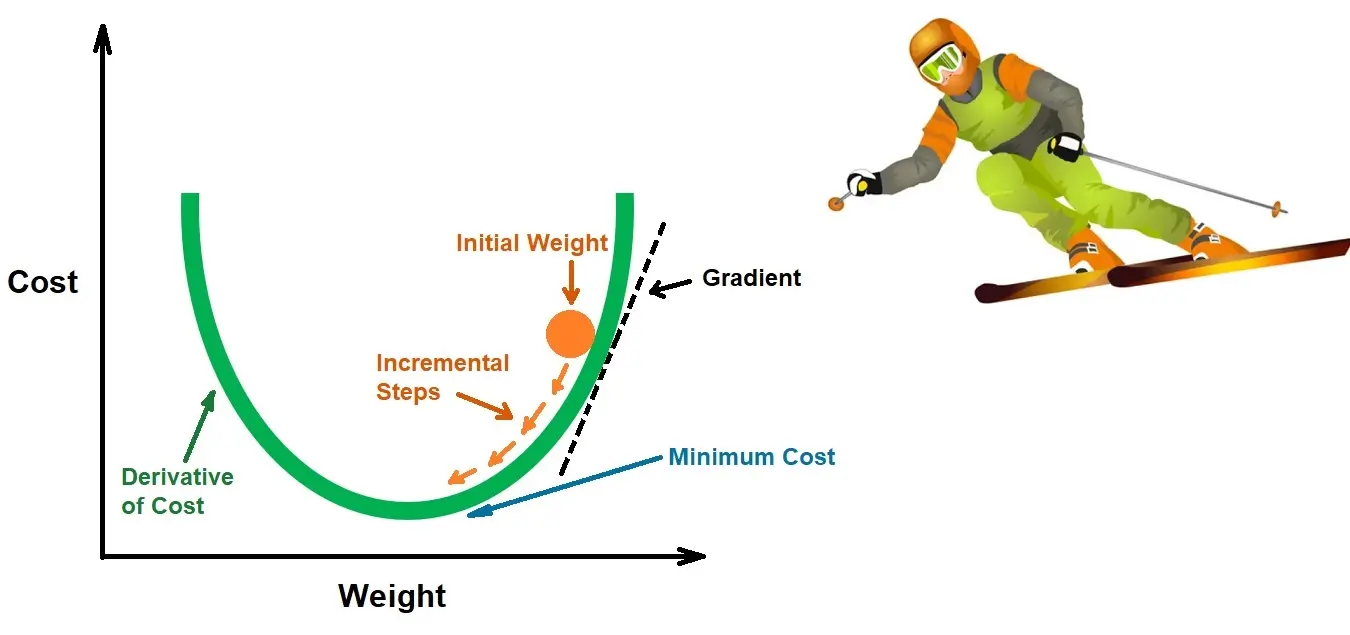
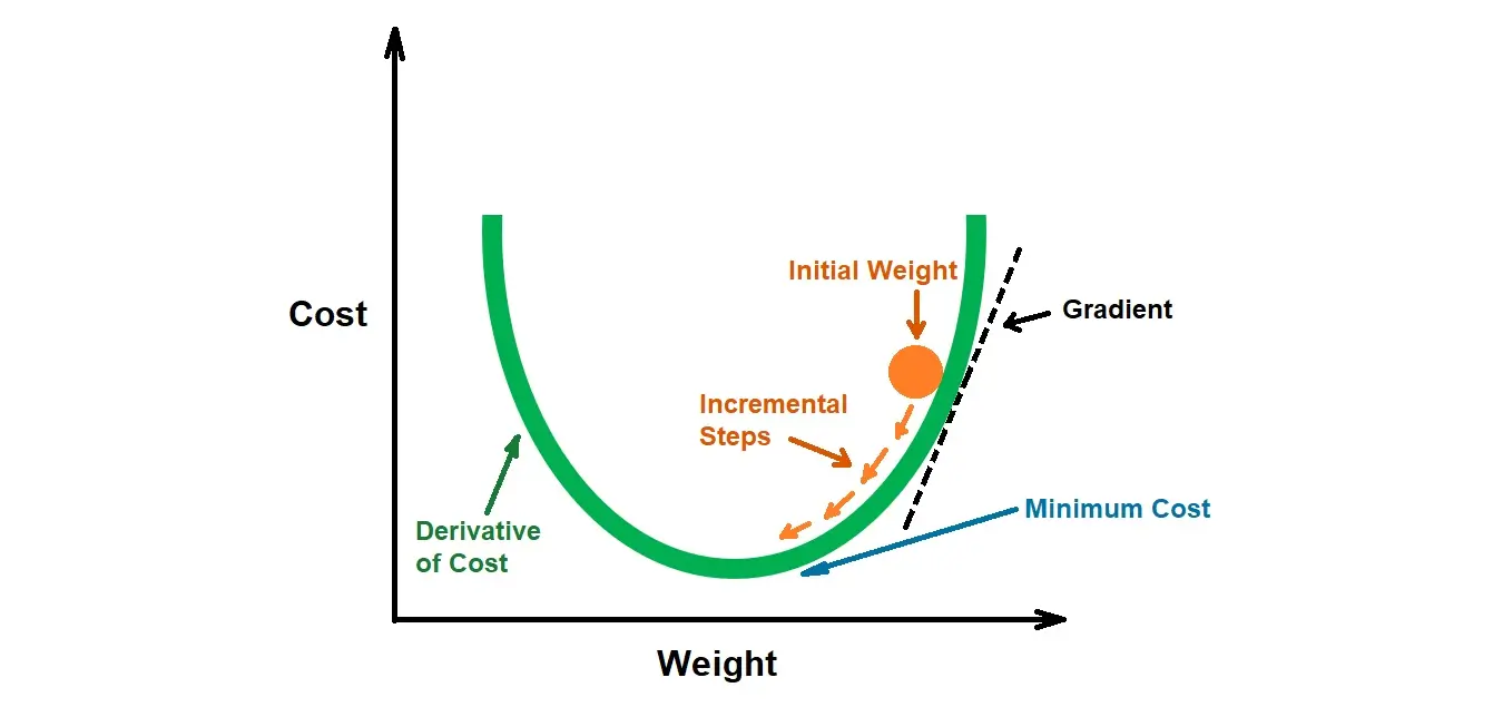
The visualization above illustrates the process, showing how Gradient Descent takes ‘incremental steps’ starting from an ‘initial weight’. At each step, the gradient is calculated, which points toward the direction of the steepest ascent. The algorithm then takes a step in the opposite direction, gradually moving towards the ‘Minimum Cost’, representing the optimal set of parameters for the model.

Key Factors Influencing Gradient Descent Efficiency

• Differentiability: Gradient Descent requires the cost function to be differentiable. A differentiable function allows the computation of the gradient, which indicates the direction of the steepest ascent. For instance, for the function f(x) = 2x² + 1, the first derivative is f'(x) = 4x, providing the gradient for Gradient Descent to determine how the function’s output changes with x.
• Convexity: The cost function should ideally be convex to ensure that Gradient Descent can reliably find the global minimum. A convex function has a second derivative that is non-negative across its domain. For the given function, f(x) = 2x² + 1, the second derivative f”(x) = 4 is positive and constant, confirming that the function is convex and suitable for Gradient Descent.

When applying Gradient Descent to the function f(x) = 2x² + 1, the update rule incorporating the derivatives becomes:

x_{n+1} = x_n – (\alpha \times 4x_n)

Here, x_n is the current estimate, x_{n+1} is the updated estimate, and α is the learning rate. This rule is iteratively applied to adjust the value of x to minimize the cost function, moving towards the point where f(x) is at its minimum.

Steps to Implement the Algorithm

• Choose a starting point for our value.
• Calculate the gradient at that point.
• Make a scaled-down movement in the opposite direction by multiplying the value by the gradient descent.
• Repeat steps 2 and 3.
• Make changes to the code.

Simple Example 

Let’s take an example using gradient descent to minimize the value of a cost function. Let’s look at our equation for the gradient of RMSE (Root-mean-square deviation)

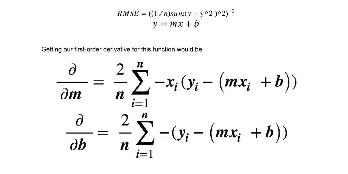
We can solve for the first-order derivative of both the m and b values.

Let’s look at the following JavaScript code for implementing Gradient Descent:

const x = [1,2,3,4,5,6,7,8,9,10];
const y = [2,4,6,8,10,12,14,16,18,20];
const calculatedValue =1000;
const learningRate = 0.01;
let slope = 400;
let startingPoint = 1
const calculateLine  = (x) =>{
  return startingPoint + (x * slope) 
}

const error = (y , calculatedValue) =>{
  return y - calculatedValue
}

const sumCostFunction  = (exludeX) =>{
  let startingPoint = 0;
  for (let i = 0; i < x.length; i++) {

    startingPoint = startingPoint + (exludeX?-1:(-1 * x[i])) * error(y[i],calculateLine(x[i],slope,startingPoint))
    
  }

  return startingPoint
}

const gradient = (exludeX)=>{
  return (2/x.length) * sumCostFunction(exludeX)
}

const calcGradient = () =>{

  for (let i = 0; i < 100000; i++) {
   
  const tempM = learningRate * gradient(true)
  const tempB = learningRate * gradient(false)

  startingPoint = startingPoint - tempM
  slope = slope - tempB

    console.log(`starting point is ${startingPoint} slope is ${slope}`)
  }

  
}

calcGradient()

Output from the Above Code

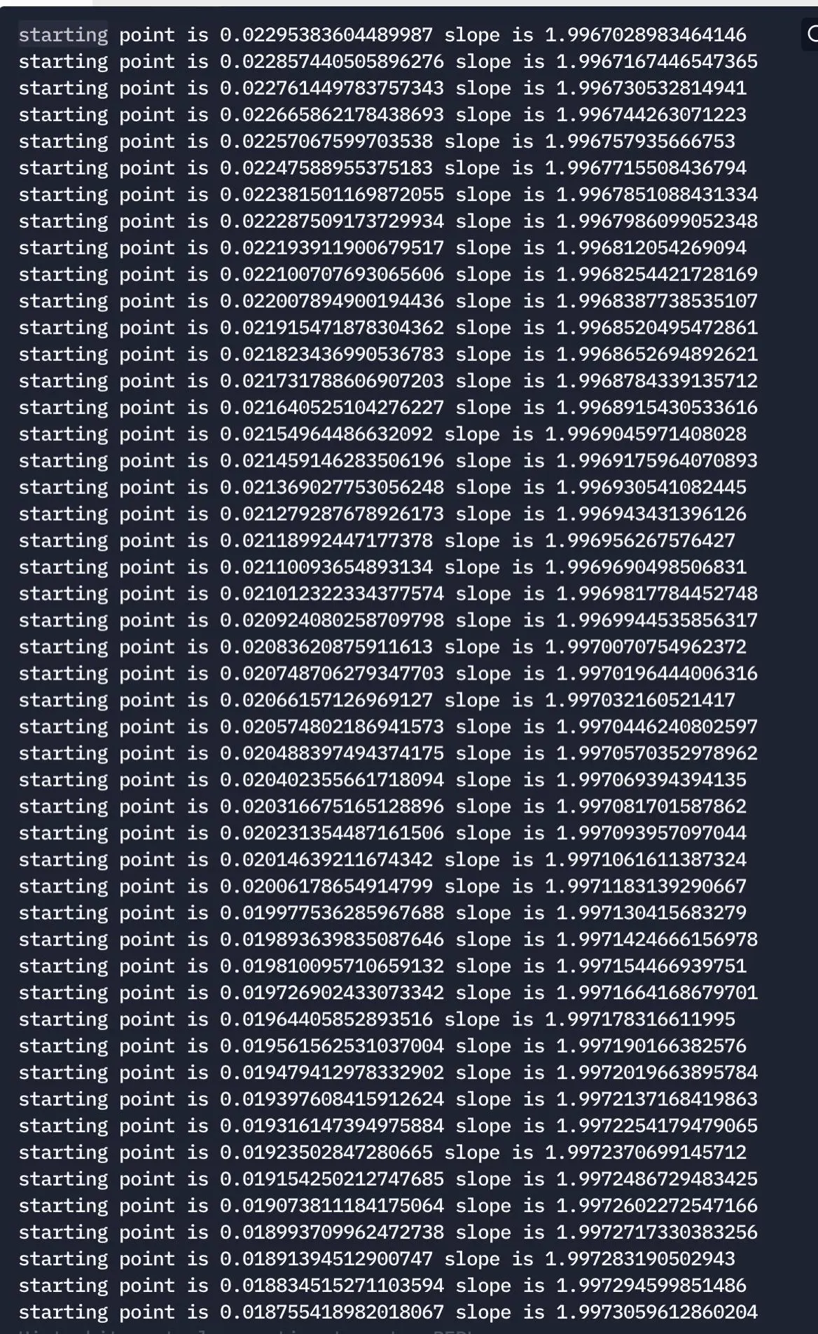
Here, we can see our dependent variables, our slope, and the starting point change after every iteration.

Conclusion 

Building out our model and training can be a breeze once we understand the math behind it and break it down into smaller, simpler steps. We learned about gradient descent and its components, why it works from a math perspective, and its implementation in JavaScript. Moving forward, we can apply this optimization to neural networks and other machine learning models.